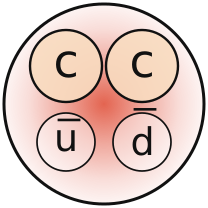
Hadron Spectroscopy
Classification and phenomenology
Mikhail Mikhasenko · Lecture 1
AEPSHEP 2026 · Taipei
25 October 2026, 09:00–10:30

Lecture 1 roadmap
A. QCD basics
B. Excited states
C. Observation of hadrons
D. Decays and the hadronic continuum
QCD basics
A · Fields, vacuum and confinement
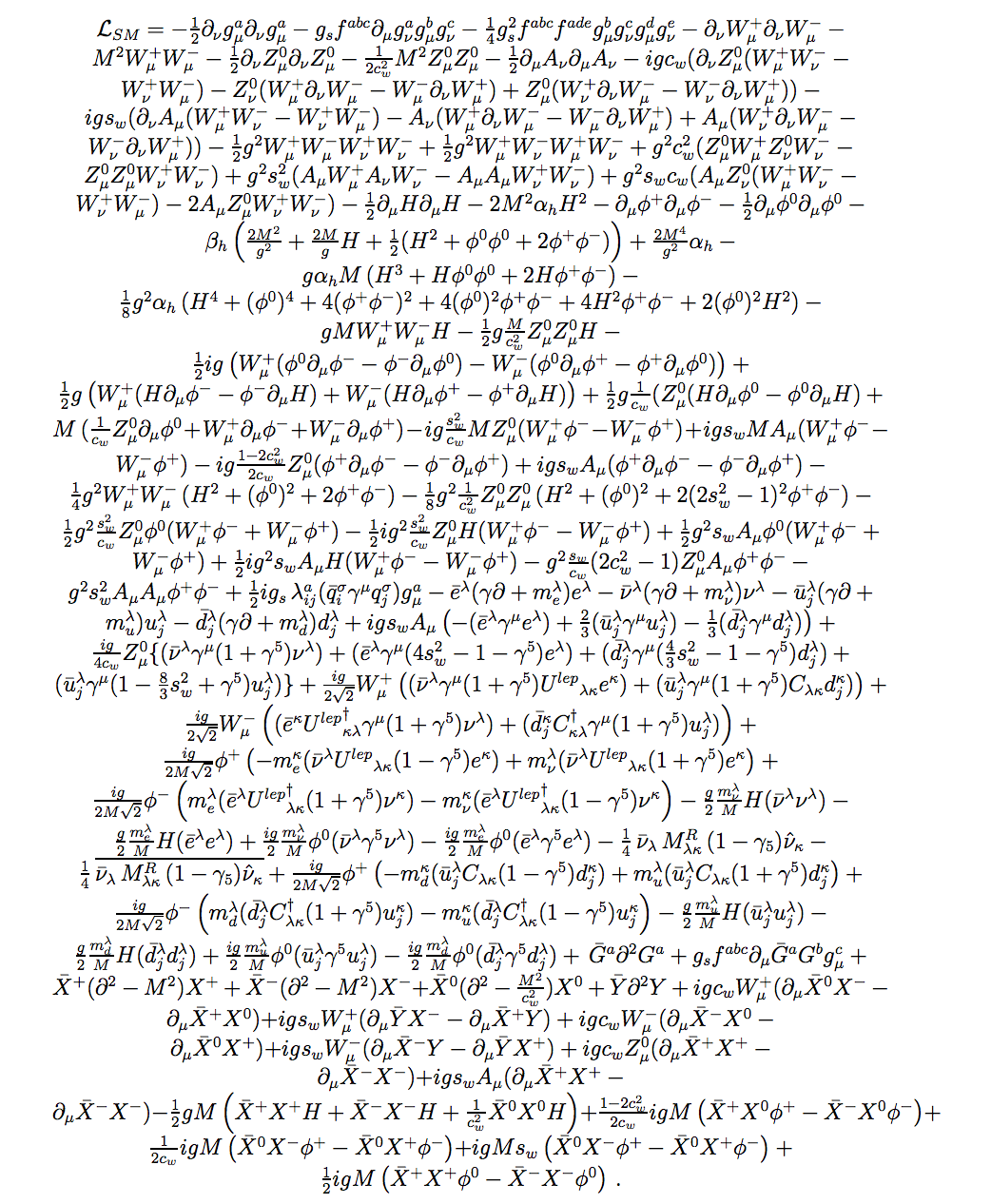
The QCD Lagrangian
Quarks carry colour
: quark of flavour ; : colour generators.
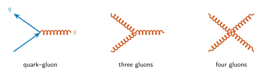
Gluons interact with gluons
Eight gluon fields, .
![TikZ diagrams of quark-gluon, three-gluon and four-gluon vertices]()
The non-Abelian term generates the three- and four-gluon vertices. Gauge-fixing and ghost terms are omitted here.
The QCD vacuum
Empty space is not empty of fields.
Even the lowest-energy state contains fluctuating chromo-electric and chromo-magnetic fields.
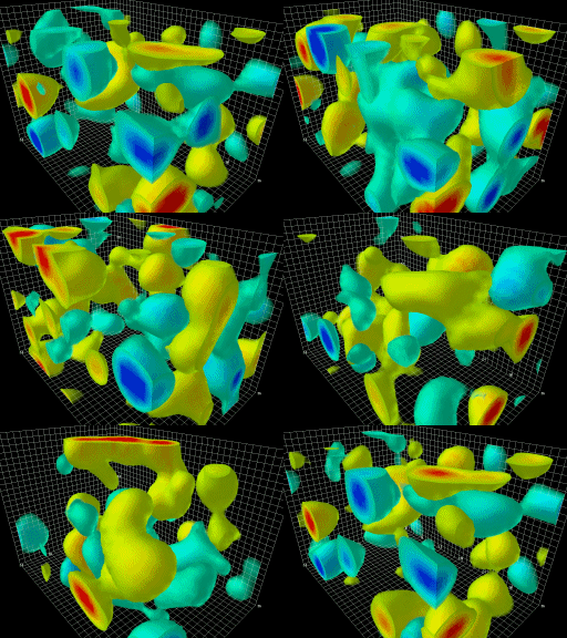
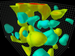
What are we looking at?
- A lattice-QCD field in a box of — a few proton sizes.
- 50 smoothing sweeps reveal the larger-scale lumps.
- Colour shows topological charge density: the local sign and strength of the field’s winding.
A view of a smoothed quantum field, not individual gluons flying through empty space. The animation is not real-time motion.
Confinement and flux tubes
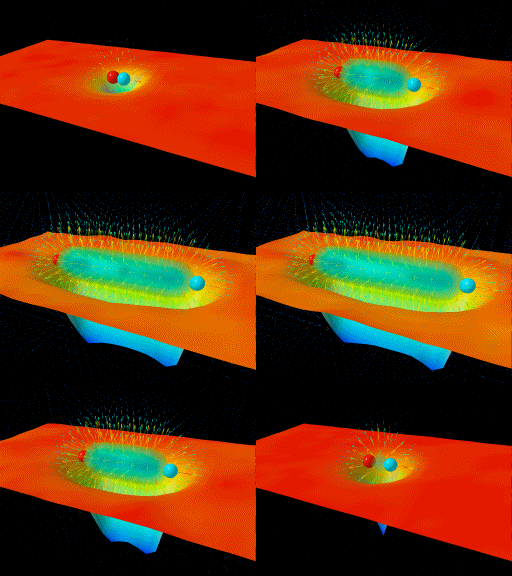
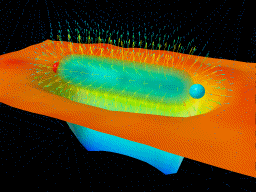
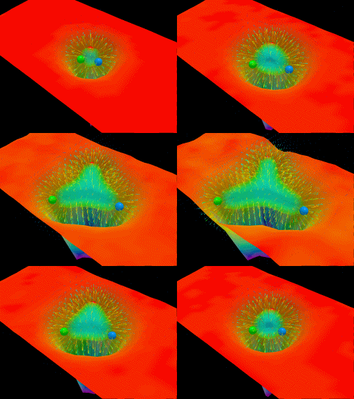
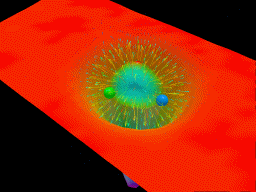
Pull the quarks apart
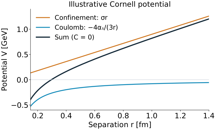
The field forms a longer tube of almost constant width. More length costs more energy.
Surfaces: reduction of vacuum action density around static sources.
sets the energy zero. With light quarks, a long string can break into two hadrons.
What field structures support confinement? Lattice studies link the linear potential to centre vortices.
Centre vortices
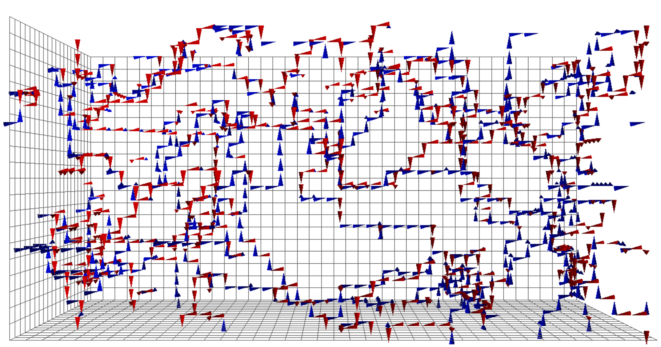
![Large lattice centre-vortex map: red and blue oriented flux segments]()
A 3D slice through the vortex network · Biddle, Kamleh & Leinweber


A familiar vortex — an analogy, not a QCD simulation.
Read the map
Lines mark centre flux; red and blue distinguish its orientation.
A 3D slice cuts the four-dimensional vortex surfaces into lines.
Remove the identified vortices in a lattice calculation → the confining linear rise disappears. Keep them → the confining behaviour survives.
Effective degrees of freedom
Gluons: self-interactions and confinement
- Light: nearly massless on hadronic scales; is heavier.
- Cheap: light quark–antiquark pairs are easier to create.
- Mixed: neutral light mesons can mix flavour components.
Heavy quarks:
()
- Massive: charm and bottom provide a large mass scale.
- Expensive: creating a heavy pair needs much more energy.
- Persistent: a heavy quark usually remains a useful label for its hadron.
Strong interactions conserve net flavour for all quarks.
The top quark decays before forming ordinary hadrons.
IIIIIIuctdsb
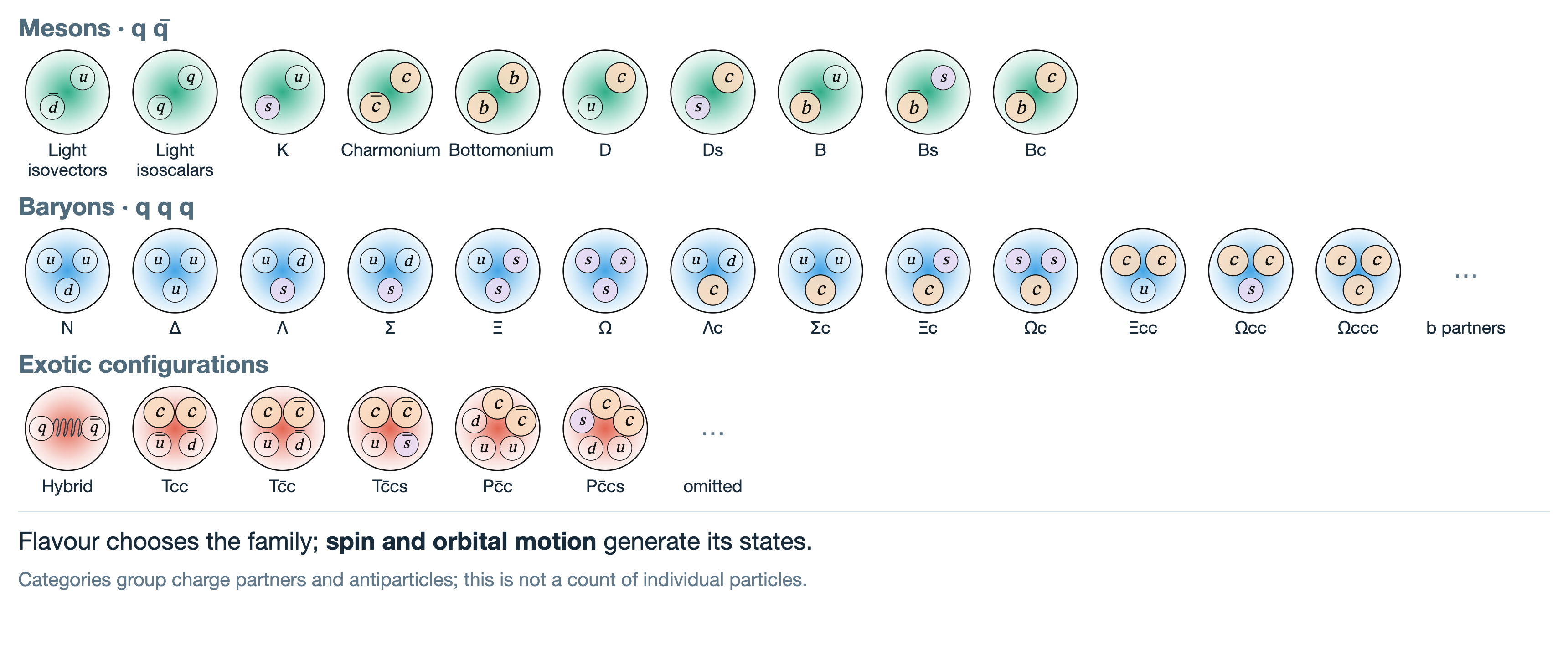
Quarks and hadron families
Excited states
B · Spin, orbital motion and excitation multiplets
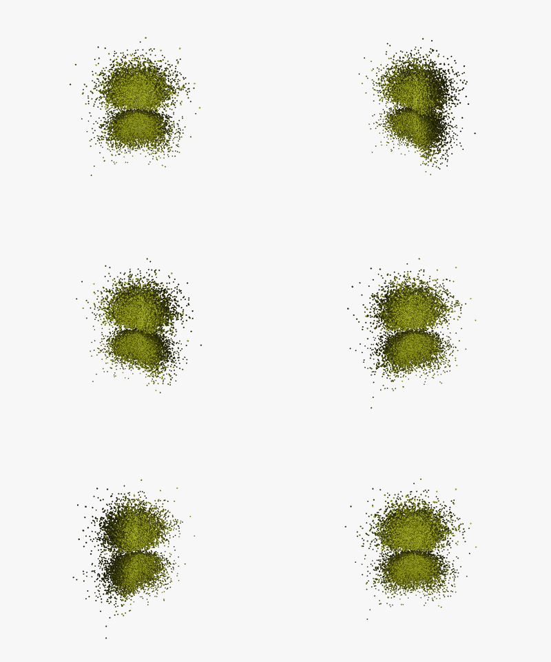
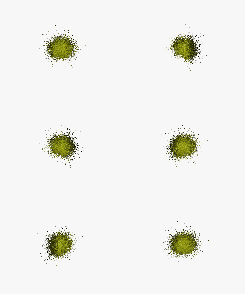
Radial and orbital multiplets
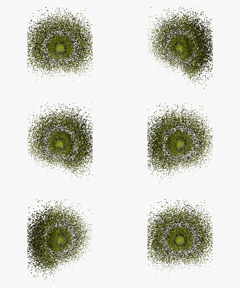
Wavefunctions and nodes
Excitation energy ↑
S · L = 0
P · L = 1
D · L = 2
3S
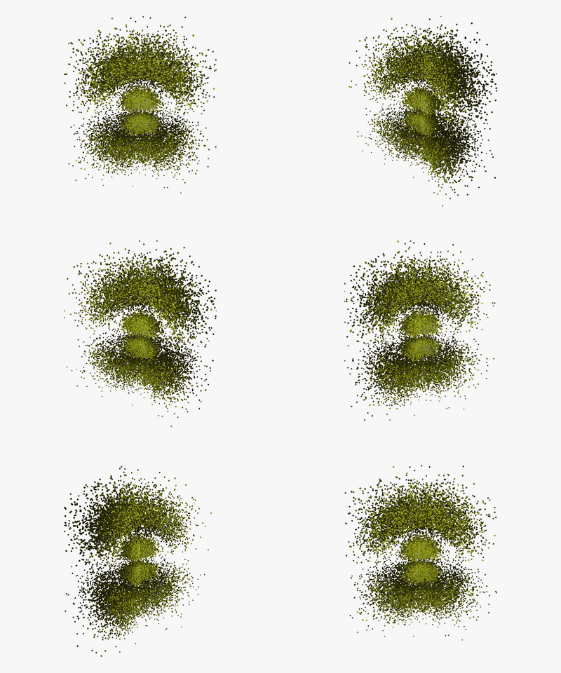
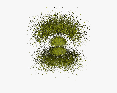
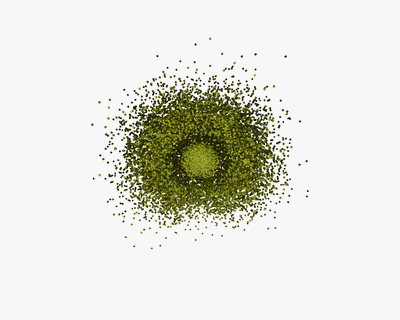
2P
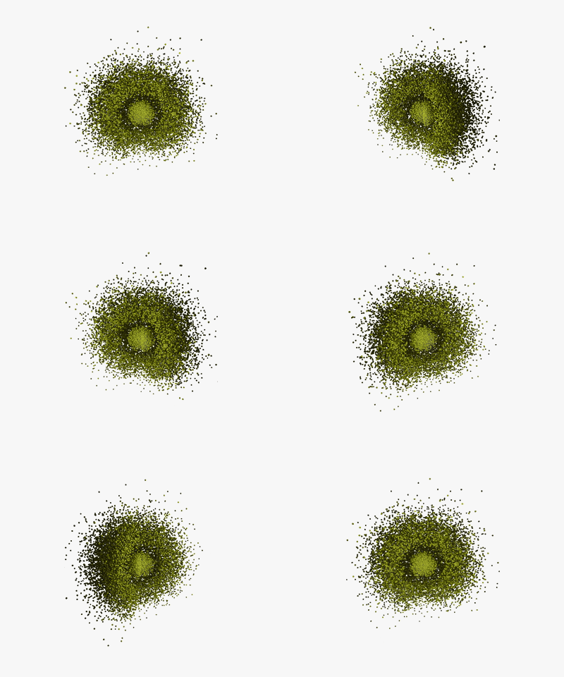
2S
1P
1S
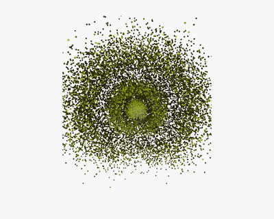
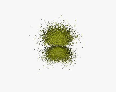
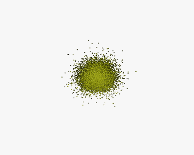
GIModel charmonium clouds · schematic energy spacings
Radial excitation
- Same orbital angular momentum .
- More nodes in the radial wavefunction.
- : 0 → 1 → 2 radial nodes.
Orbital excitation
- Increase : S → P → D.
- Change the angular shape of the wavefunction.
- The displayed P waves have an angular nodal plane.
Connection to hydrogen
, while our radial label is .
Confinement lifts the Coulomb degeneracy: and need not coincide.
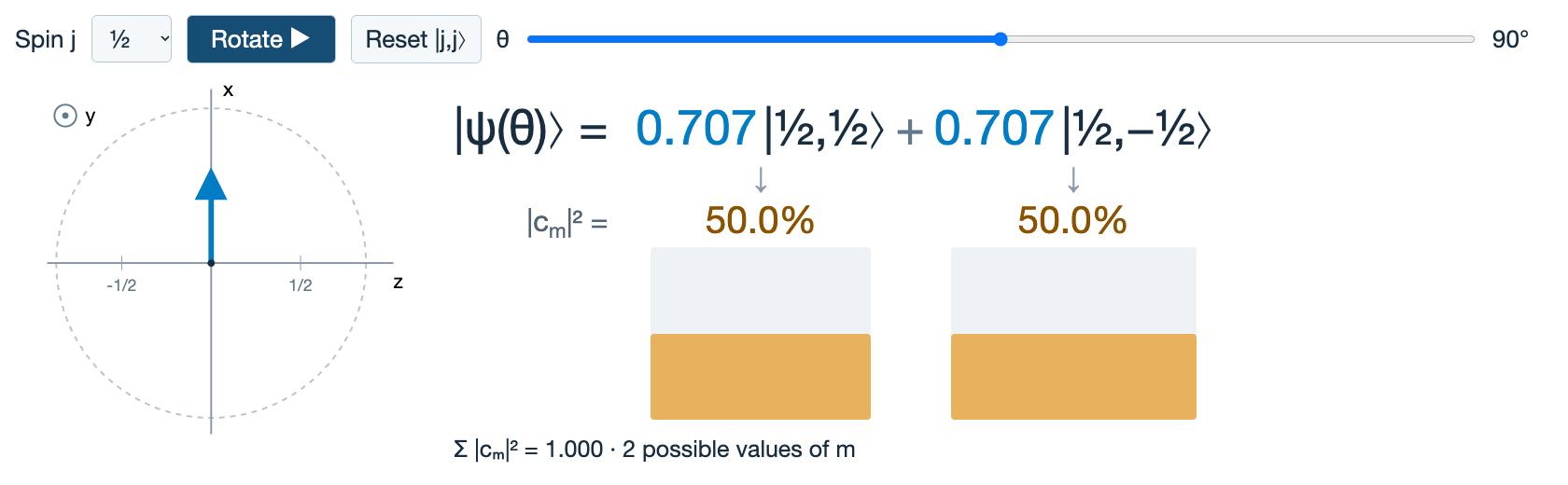
Spin and spin projection
Fixed spin ; possible projections: .
Adding two spins
1 · Add angular momenta
Vector addition — with quantized total angular momentum.
2 · Find the allowed total spins
increases in steps of one. Each value labels a separate multiplet.
3 · Then resolve the projections
For each , there are states:
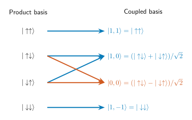
Example: singlet and triplet
![Coloured TikZ transformation of two spin-half product states into singlet and triplet states]()
Triplet : symmetric under exchange.
Three projections: .
Singlet : antisymmetric under exchange.
One projection: .
Spin and orbital motion
³⁄₂+ ⊗ ½−
S = 1 ladder
S = 2 ladder
Relative motion
1−
2−
S wave L = 0
0+ 1+ 2+
1+ 2+ 3+
P wave L = 1
1− 2− 3−
0− 1− 2− 3− 4−
D wave L = 2
2+ 3+ 4+
1+ 2+ 3+ 4+ 5+
F wave L = 3
Each initial generates its own orbital ladder. Repeated values in different columns are distinct coupled configurations.
Meson quantum numbers
For a neutral, self-conjugate state, charge conjugation exchanges quark and antiquark.
Parity: P = (−1)L+1Charge conjugation: C = (−1)L+S
½+ ⊗ ½−
S = 0 ladder
S = 1 ladder
Relative motion
0−+
1−−
S wave L = 0
1+−
0++ 1++ 2++
P wave L = 1
2−+
1−− 2−− 3−−
D wave L = 2
3+−
2++ 3++ 4++
F wave L = 3
Forbidden for conventional q q̄: 0−−, 0+−, 1−+, 2+−, 3−+, …
Isospin
u ↔︎ dNearly equal masses on the strong-interaction scale.
QCD treats them almost identically → approximate isospin symmetry.
The same addition rules as spin
One light quark forms a doublet:
Three light quarks:
Nucleons: →
Delta baryons: →
Here “light” means u or d. The quarks are isospin singlets: .
Neutral mesons: equal-weight mixtures
The and flavour configurations mix into states of definite isospin:
Isoscalar ·
Isovector ·
Maximal mixing: equal magnitudes, with a plus or minus relative sign.
Nearly degenerate members of each multiplet — not necessarily equal masses for the and multiplets.
Baryons: good and bad diquarks
Heavy quark:
Light pair: internal S wave, colour
Good diquark
Antisymmetric flavour
Bad diquark
Symmetric flavour
Relative : , .
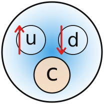 Λc · good
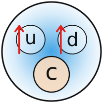 Σc · bad (isospin)
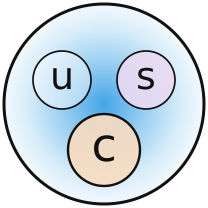 Ξc, Ξ′c · good + bad
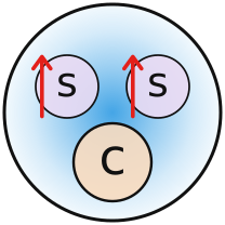 Ωc · bad (identity)
A heavy quark and a good diquark
For with and relative , which levels are allowed?
A. only
B. only
C.
D. only
A heavy quark and a bad diquark
For with and relative , which levels are allowed?
A. only
B. only
C.
D.
Can the good diquark be uu?
For an internally S-wave, colour- pair, which spin is compatible with Fermi statistics?
A. only
B. only
C. Both and
D. Neither
Hyperfine splitting
For two spin- constituents:
With a fixed spatial wavefunction,
Vary : the singlet and triplet separate while the spin-weighted centroid stays fixed.
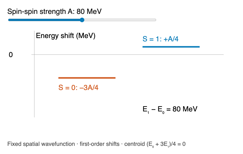
Exact spin algebra; illustrative first-order model. Full GIModel spectra follow.
Quark Model calculation
One relativized Hamiltonian
18 shared parameters → light, heavy–light and heavy-quarkonium families.
Cornell potential: attraction + confinement
Relativistic motion and spin interactions
GI adds running coupling, smearing and relativistic factors.
Radial:
Orbital:
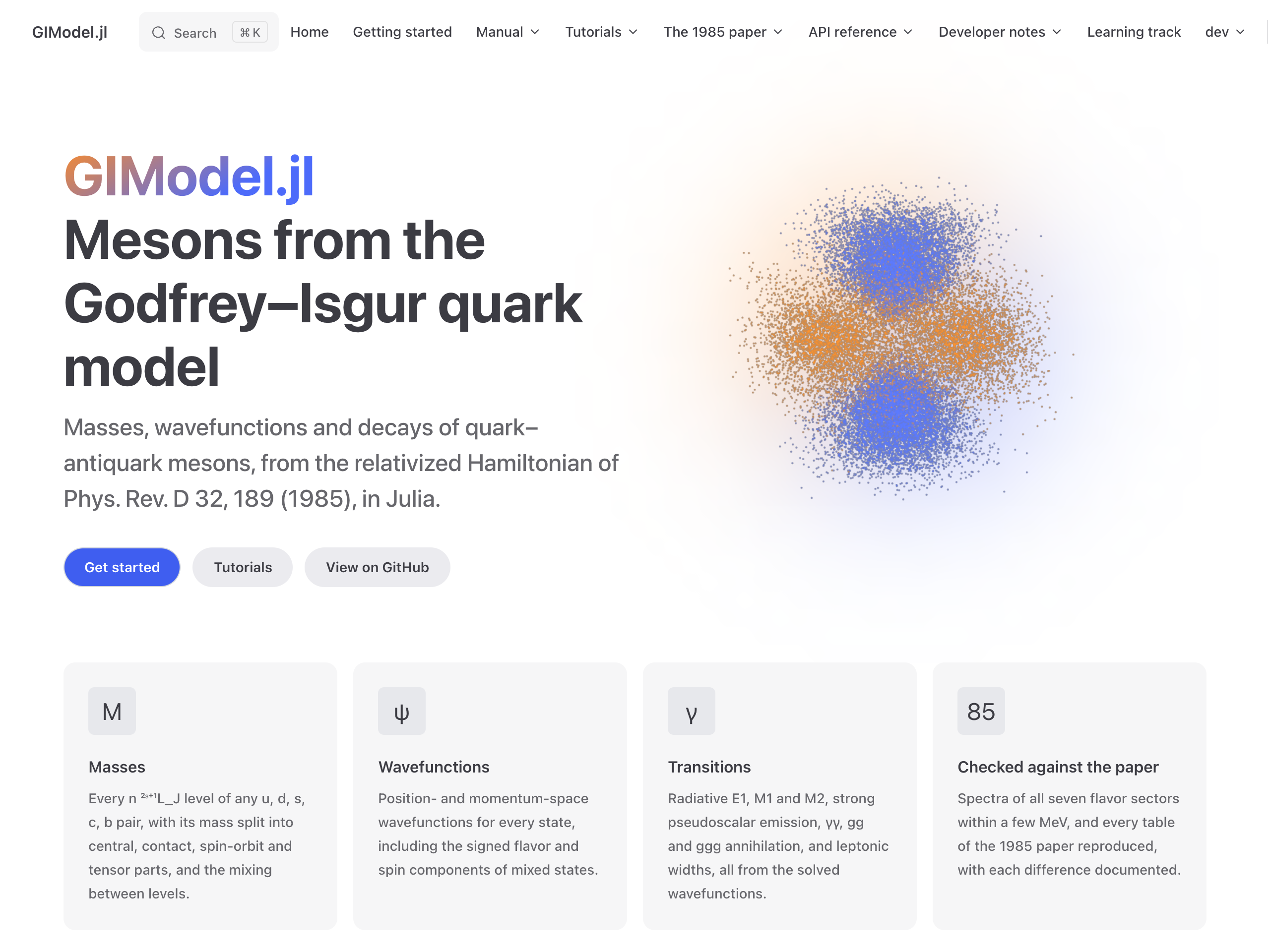
![Screenshot of the GIModel.jl documentation home page, with the wavefunction cloud and model capabilities]()
GIModel.jl · masses, wavefunctions and transitions
Building a meson family
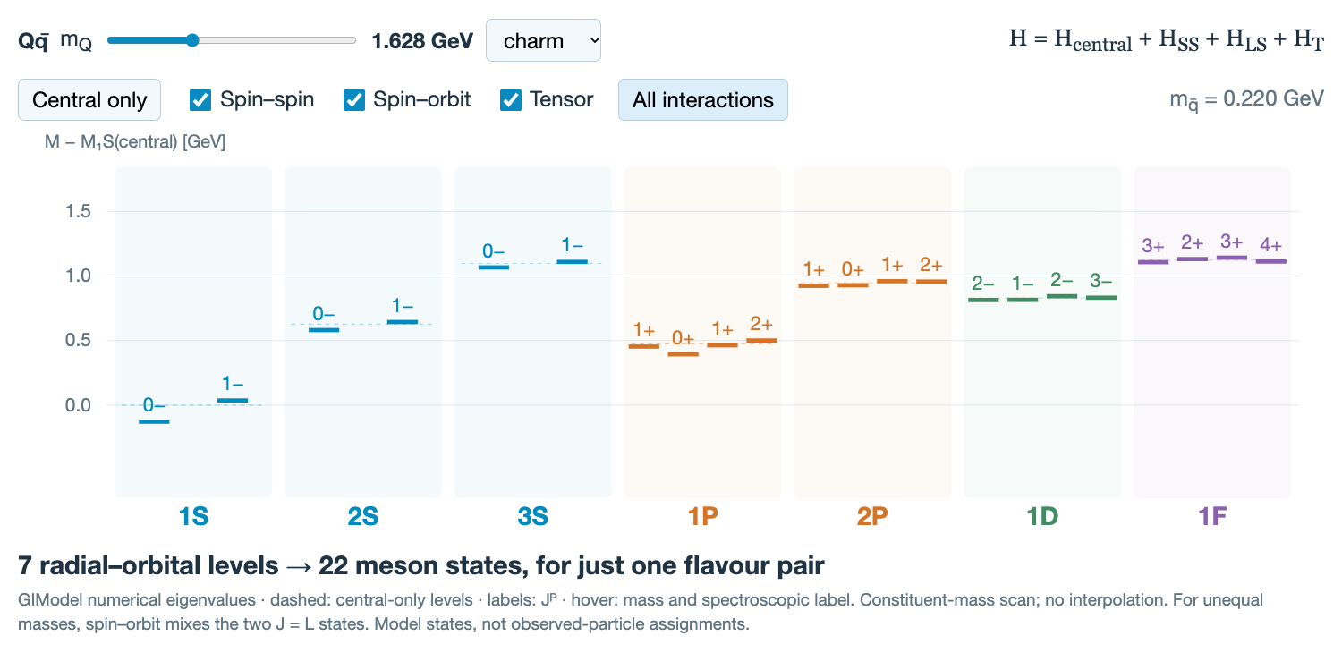
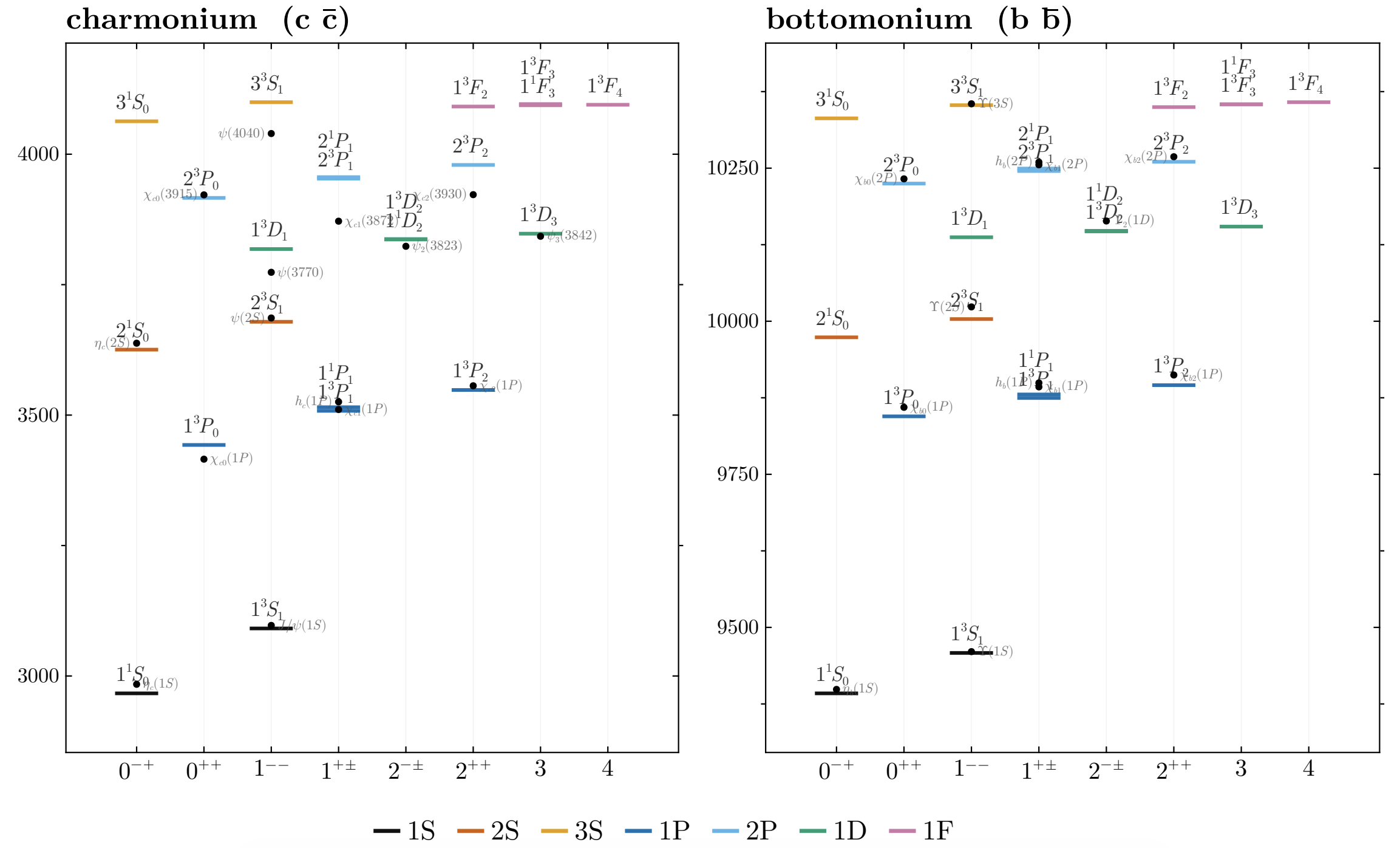
Quarkonium spectra
![User-supplied charmonium and bottomonium comparison, showing calculated excitation multiplets and named measured states]()
Observation of hadrons
C · Production, discoveries and the experimental spectrum
How we search for hadrons
Direct (prompt) production
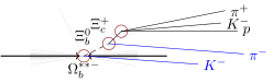
![Prompt Omega b excitation at the proton collision vertex decays to Xi b zero and K minus; Xi b and Xi c decay at displaced vertices]()
Reconstruct the long-lived and combine it with a kaon from the collision vertex.
Search for peaks in .
The resonance is prompt; its weakly decaying daughters travel before decaying.
Production in decays
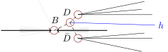
![A B meson flies from the collision vertex and decays to D, anti-D and a bachelor hadron; the charm mesons then decay at separate vertices]()
Reconstruct a displaced decay and inspect the invariant masses of its daughter pairs.
The channel reveals the structures.
Weak -hadron decays similarly probe lighter hadron resonances.
Observed hadrons: the experimental inventory
The particle physicist’s reference book
Photo: PDG · 2024 edition
From a spectrum to a catalogue
Masses, widths, quantum numbers and decay modes bring experimental results together.
756 hadron entries
Including “Further States”: some entries are less established or controversial.
Not all entries have the same level of experimental support.
A century of hadron discoveries
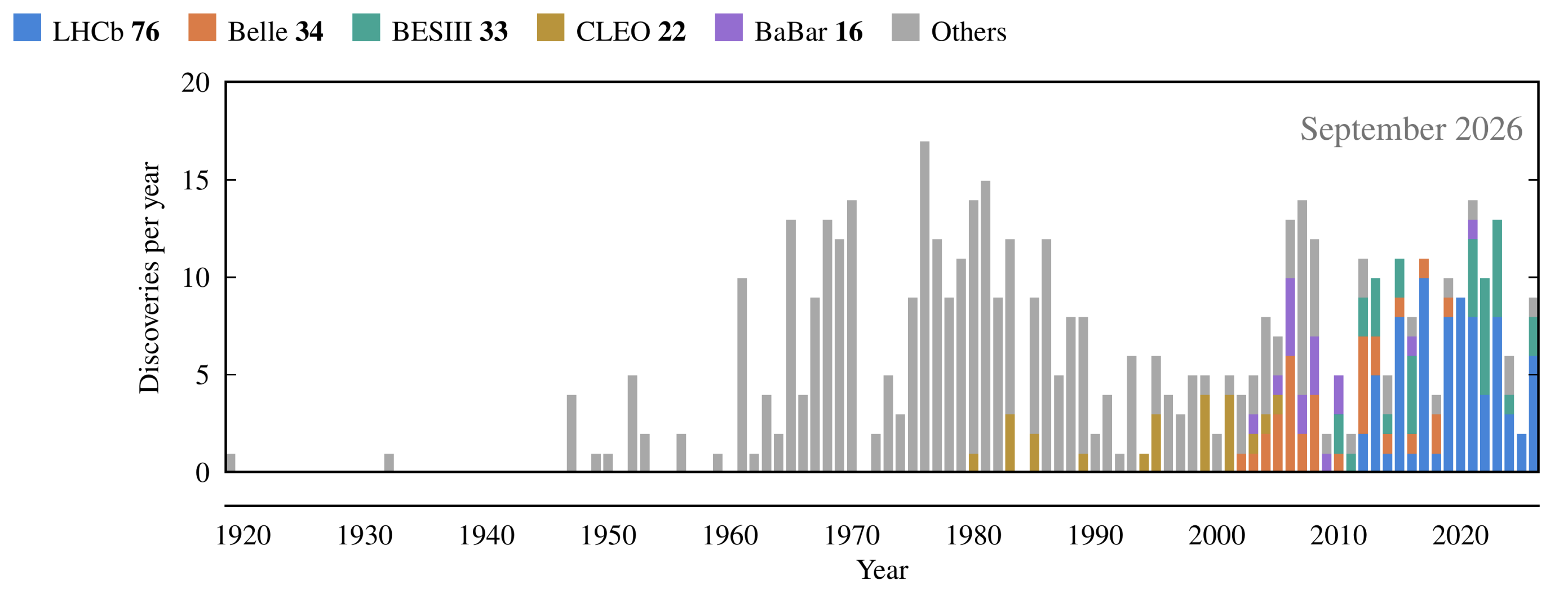
New beams and detectors keep revealing new states.
Where the discoveries happened
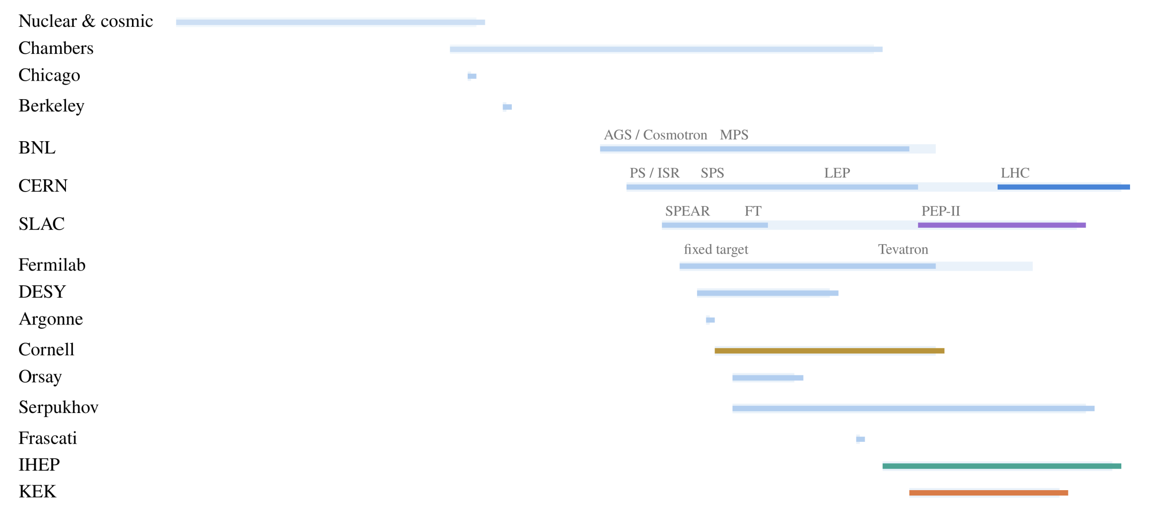
Bars span each machine’s first to last discovery—not its operating lifetime.
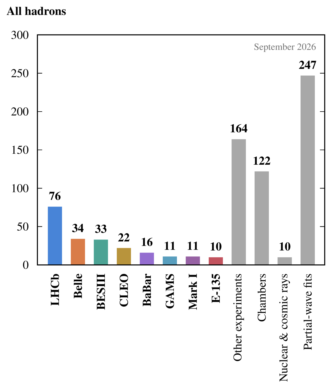
Discoveries also come from amplitude analyses
Not every state is an isolated peak
Overlapping resonances can require a partial-wave analysis to separate their contributions.
LHCb discoveries also use amplitude analyses—for example, the J/ψϕ states and hidden-charm pentaquarks.
The bars show discovery attribution, not the analysis method. “Partial-wave fits” is not the total number of states found using such fits.
Heavy-flavour baryons: organise the families
A heavy quark plus two light quarks: Qqq, Q = c or b
|
Light-quark pair
|
Charm families
|
Bottom families
|
|
ud · isospin 0
|
Λc
|
Λb
|
|
uu, ud, dd · isospin 1
|
Σc, Σc*
|
Σb, Σb*
|
|
us or ds
|
Ξc, Ξ′c, Ξc*
|
Ξb, Ξ′b, Ξb*
|
|
ss
|
Ωc, Ωc*
|
Ωb, Ωb*
|
Each flavour family can support a ladder of orbital and radial excitations.
Family labels, not a checklist of observed states. Here * denotes the spin-3/2 ground-state partner.
Resolving excited Ω baryons
Charm · css · 2017
Reconstruct Ξc⁺ K⁻: five narrow peaks.
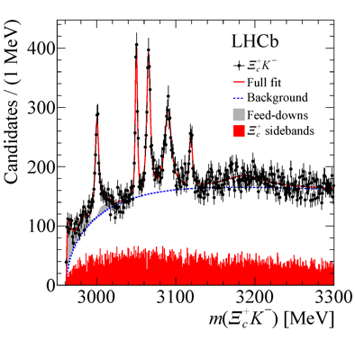
Ξc⁺ → p K⁻ π⁺
Bottom · bss · 2020
Reconstruct Ξb⁰ K⁻: four narrow structures.
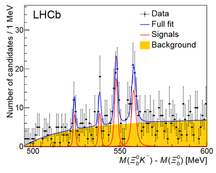
Ξb⁰ → Ξc⁺ π⁻, followed by Ξc⁺ → p K⁻ π⁺
Two heavy quarks: the Ξcc⁺⁺ discovery
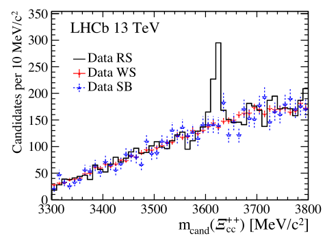
Reconstruct a weak-decay chain
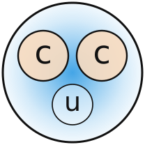
Quark content: ccu.
A narrow signal near 3621 MeV.
Check alternative charge combinations and Λc sidebands: the peak is absent.
A historical milestone in 2017: a baryon containing two charm quarks.
New hadrons at the LHC
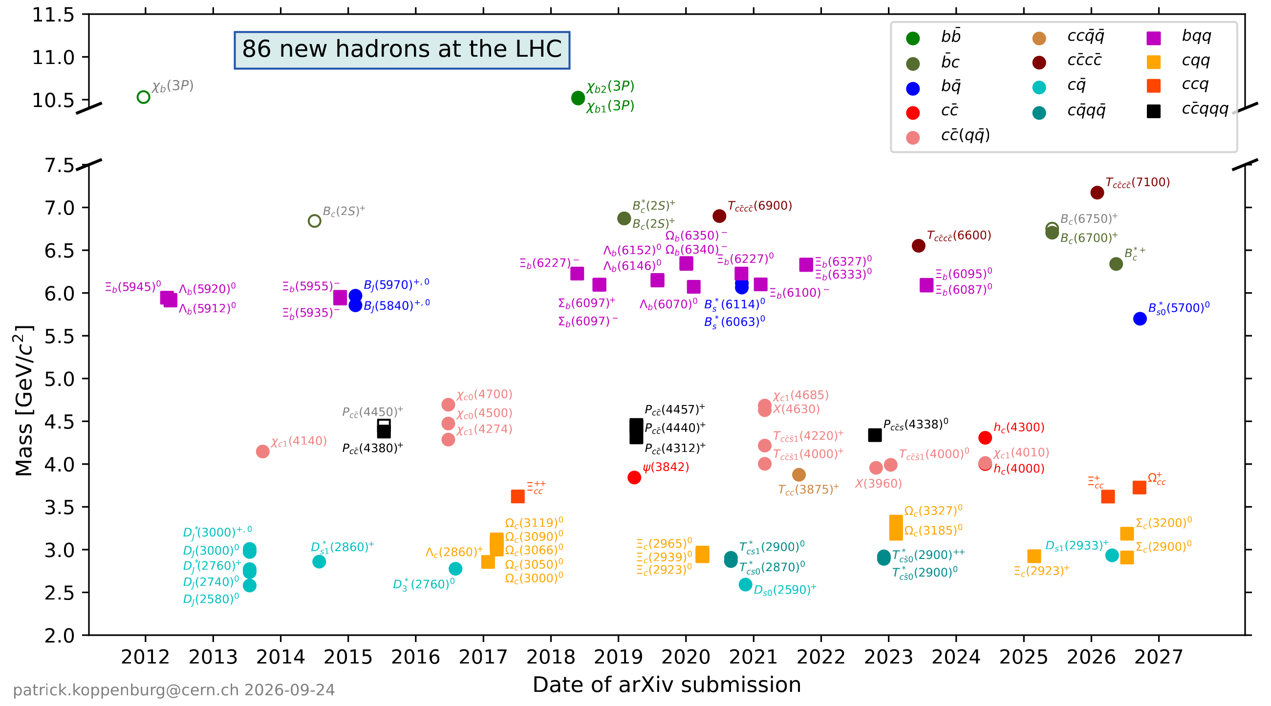
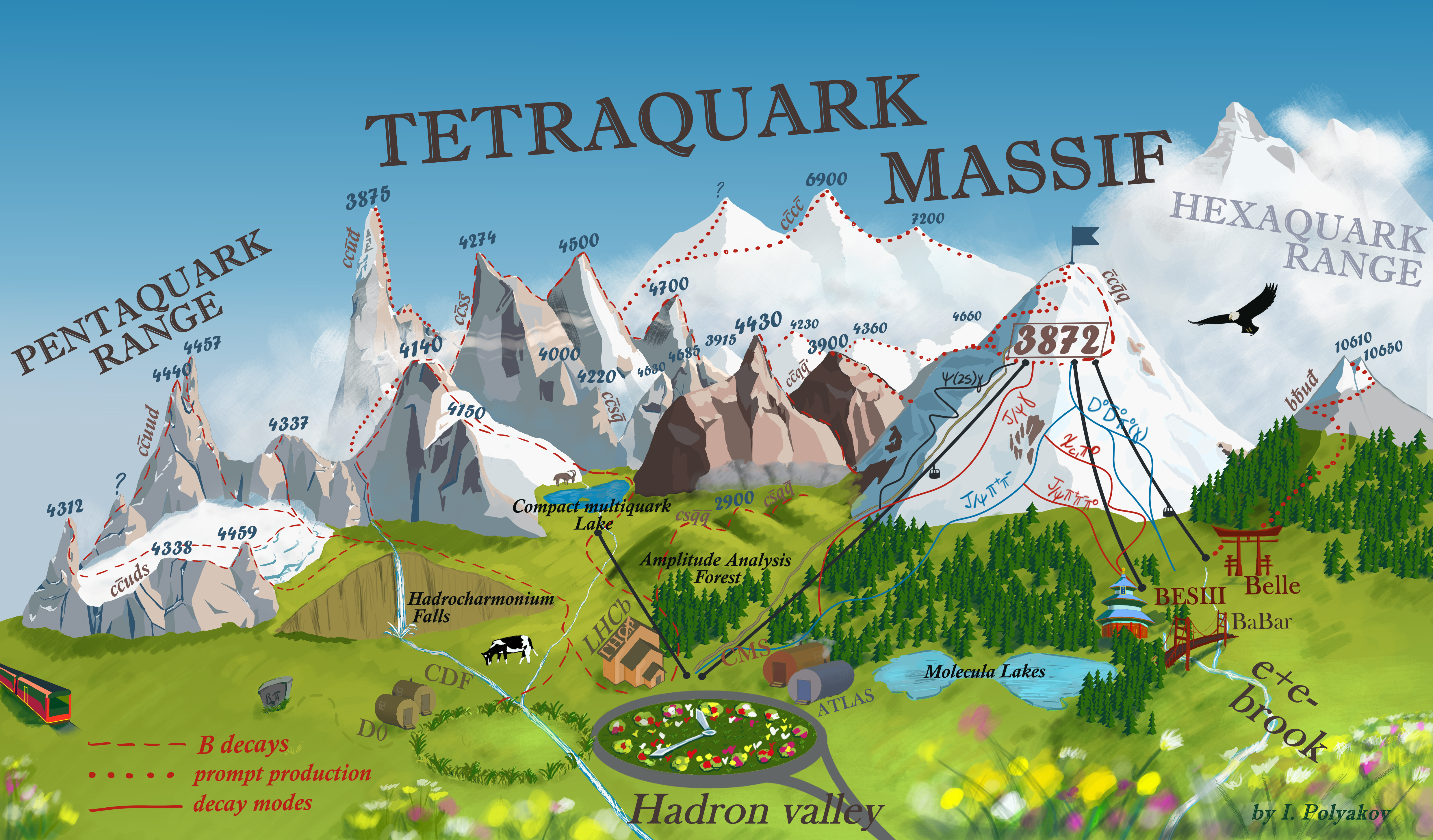
Exotic hadrons at the LHC
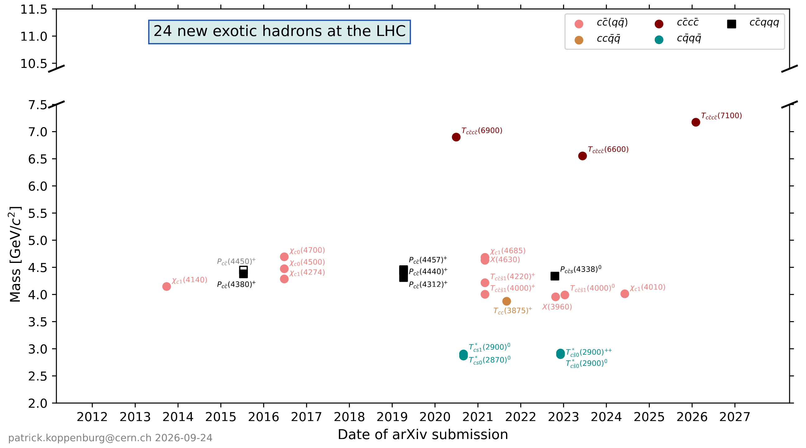
The exotic-hadron landscape
Decays and the hadronic continuum
D · Resonances, thresholds and exotic hadrons
QCD states as resonances
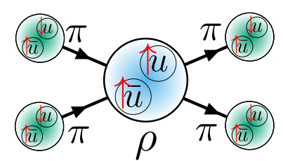
Most excited hadrons can decay through the strong interaction:
The same quantum numbers belong to a two-hadron continuum: the pair can carry any relative momentum.
A short-lived excitation appears in the interaction of these hadrons — for example, .
For an isolated, narrow resonance,
Resonances
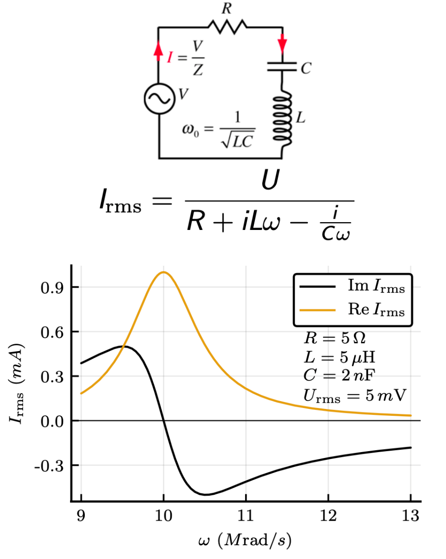
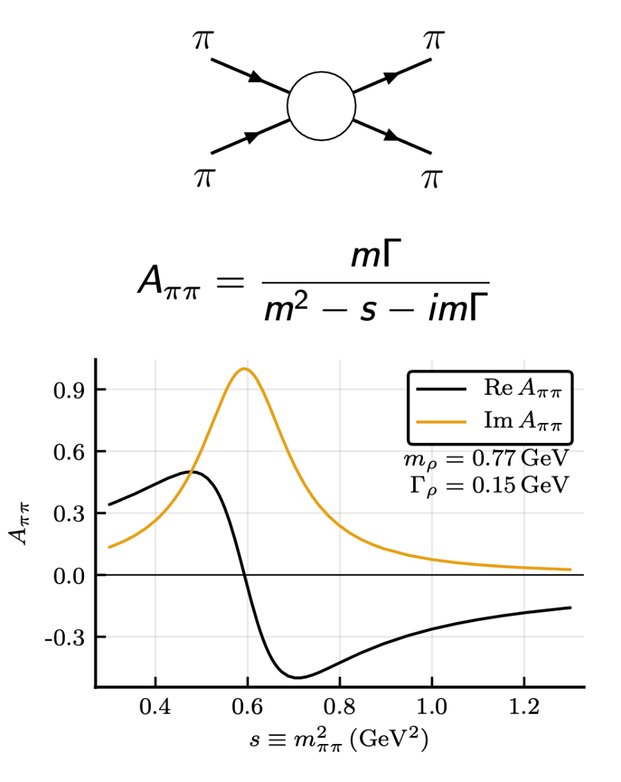
An oscillating circuit and a hadronic system share the same language:
Enhanced response near a characteristic energy.
Phase motion as the energy passes through it.
A pole of the complex response function.
Interference can turn a resonance peak into a dip.
Hadronic amplitude
The experiment measures an intensity
: final-state kinematics; : detection efficiency.
Amplitudes for the same final state interfere before squaring.
A simple resonance model
The production process changes ; the resonance pole is shared between reactions.
What goes into the width?
Far from relevant thresholds: a constant can approximate the imaginary term.
One important channel: retain , with two-body phase space .
Several channels: sum their contributions, .
Near a threshold, phase space varies rapidly. A constant-width peak can be misleading.
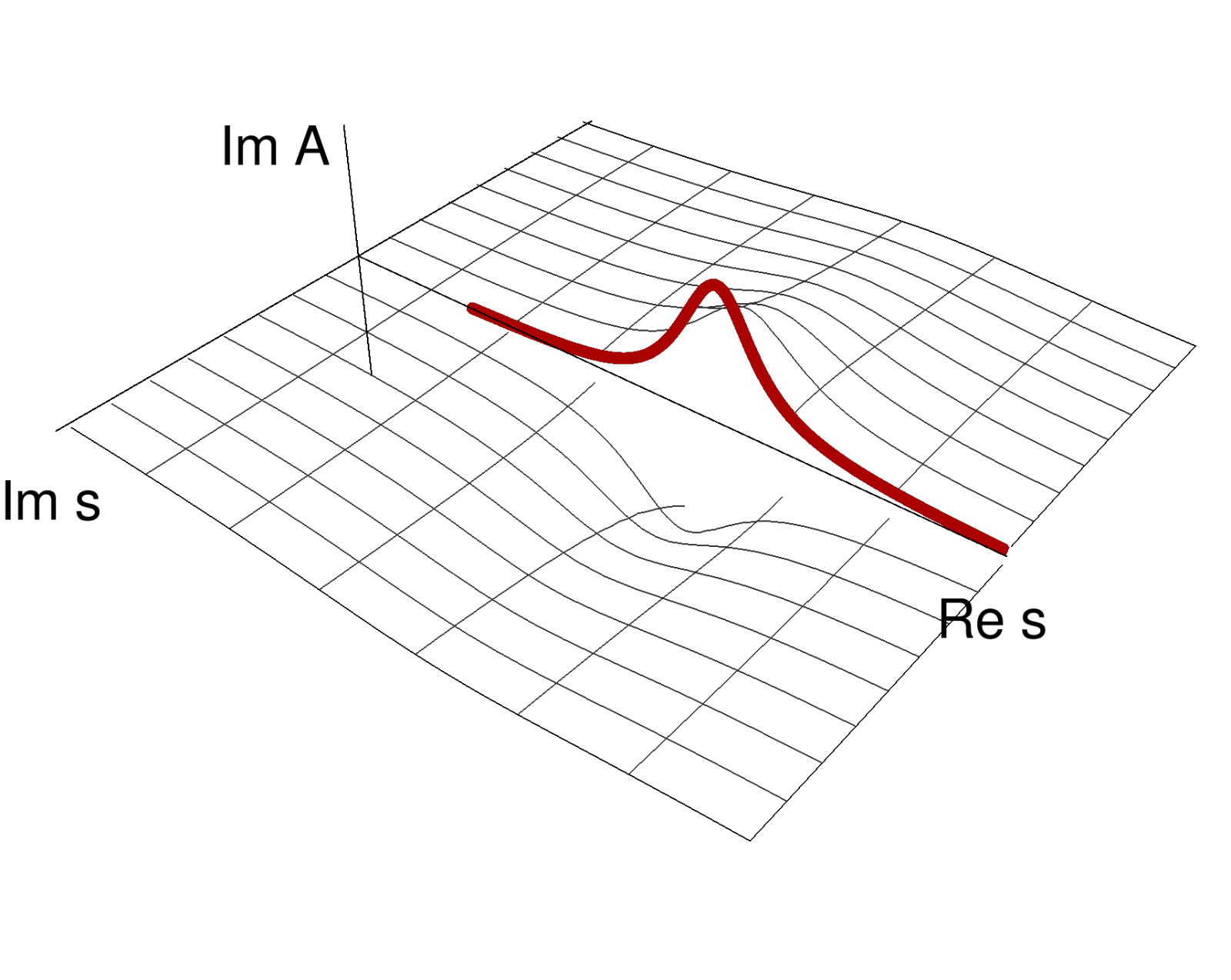
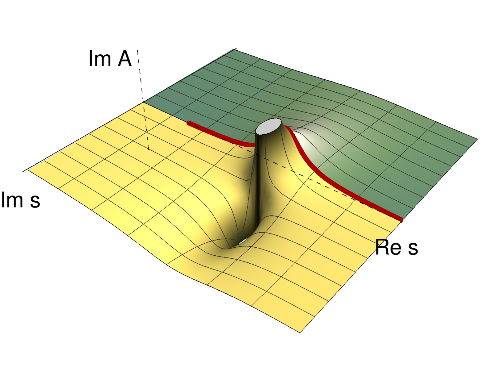
The amplitude in the complex plane
What is A?
A transition amplitude (matrix element) for chosen initial and final channels, projected onto a fixed partial wave.
The angular dependence has been projected out; channel and spin labels are suppressed.
What is s?
The invariant mass squared of the system whose resonance we study.
Analytic continuation: extend the same analytic amplitude away from real , respecting its singularities and branch choices.
can already be complex for real .
Guiding principles for amplitudes
I
Analyticity ← Causality
Causal dynamics constrains how the amplitude extends into complex energy.
II
Unitarity ← Probability conservation
Probability is conserved when all accessible final channels are included.
III
Crossing symmetry
Related reactions are described by continuations of the same underlying amplitude.
Consequences: analytic structure
- Hadronic resonances → poles on unphysical sheets.
- Decay-channel thresholds → branch points, joining a non-trivial set of Riemann sheets.
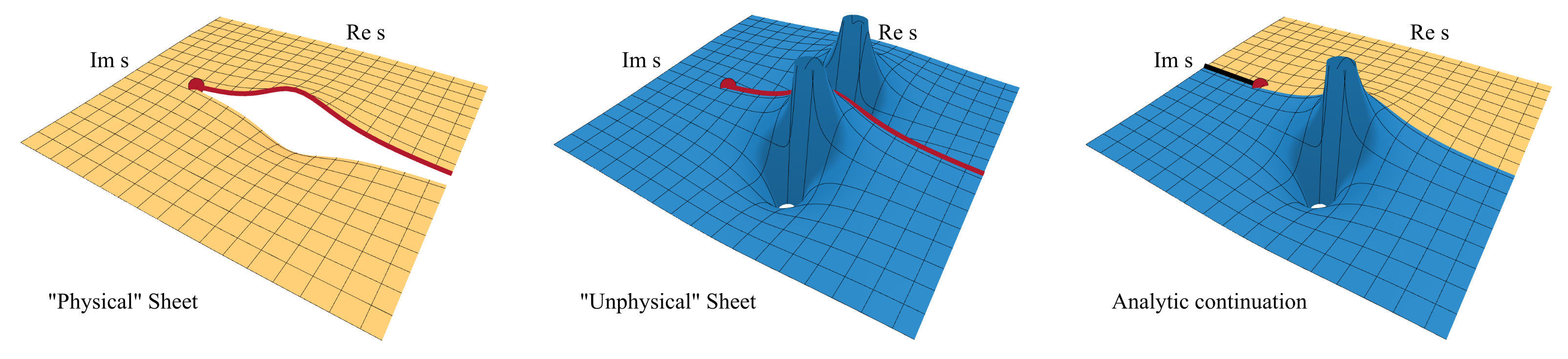
First and second Riemann sheets
![Figure 6 from Hanhart and Mikhasenko: physical sheet in gold, second sheet with resonance poles in blue, and their analytic connection]()
Physical sheet
The red curve follows the physical real-energy axis.
Second sheet
Resonance poles influence the amplitude on the physical axis.
Analytic continuation
The upper physical sheet joins the lower second sheet across the cut.
A threshold is a branch point: the two signs of the square root lead to two sheets.
Let’s play the game
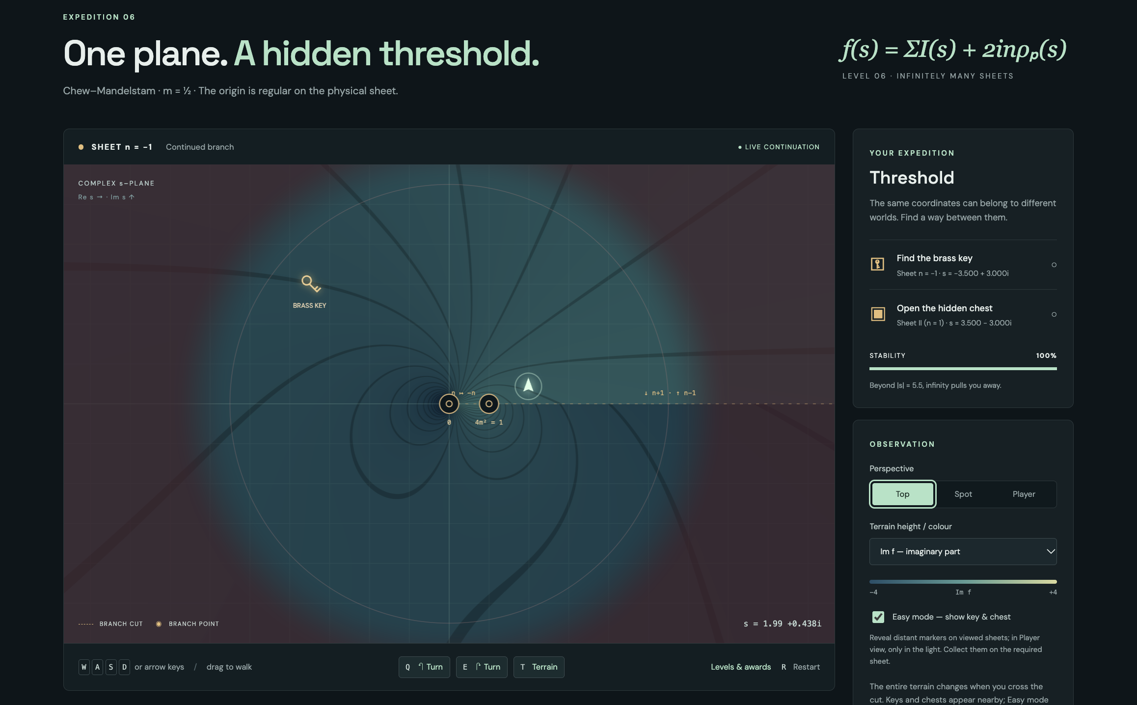
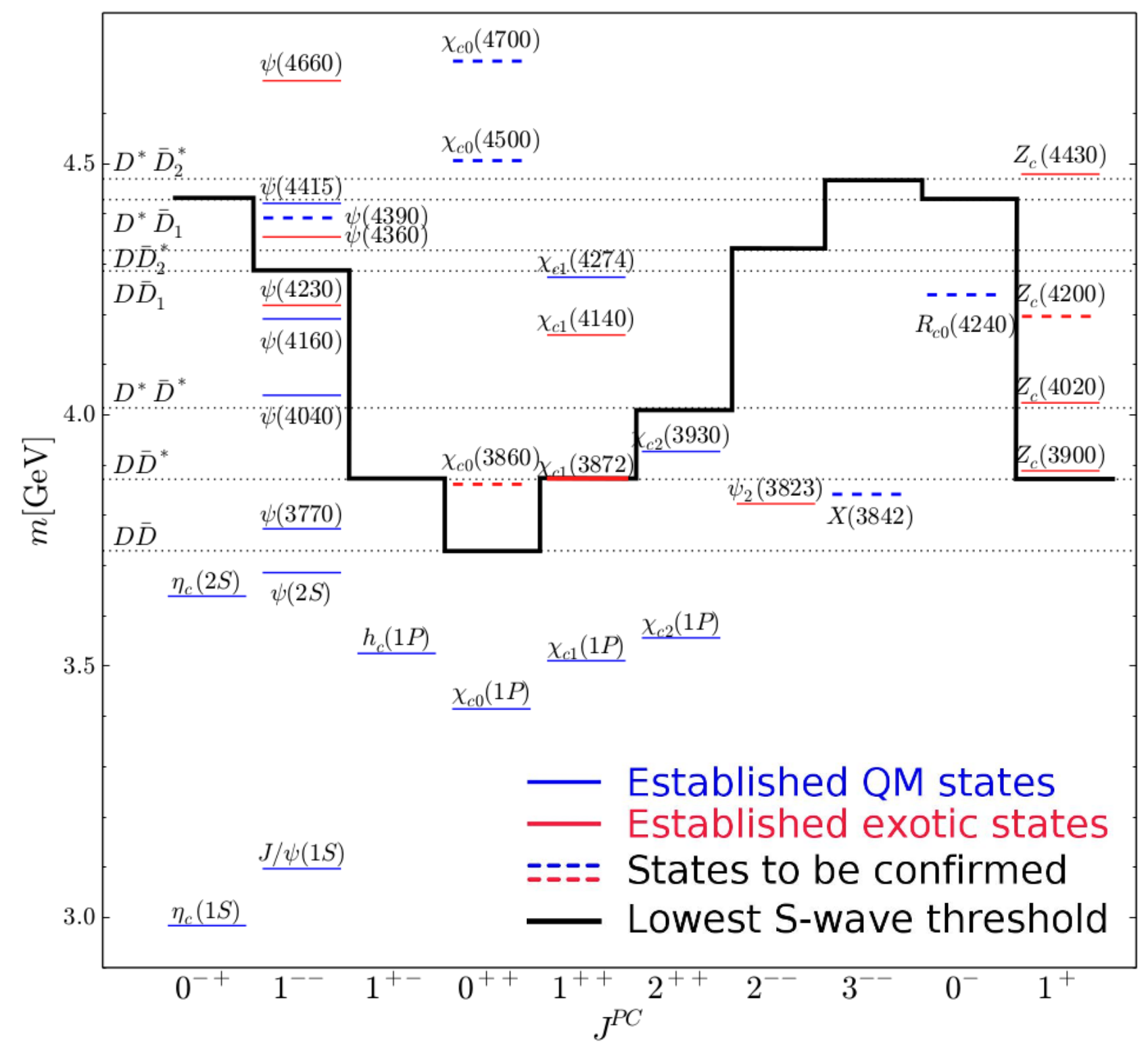
Quark-model states and thresholds
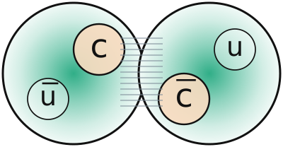
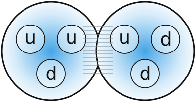
Why a molecule can be a good model
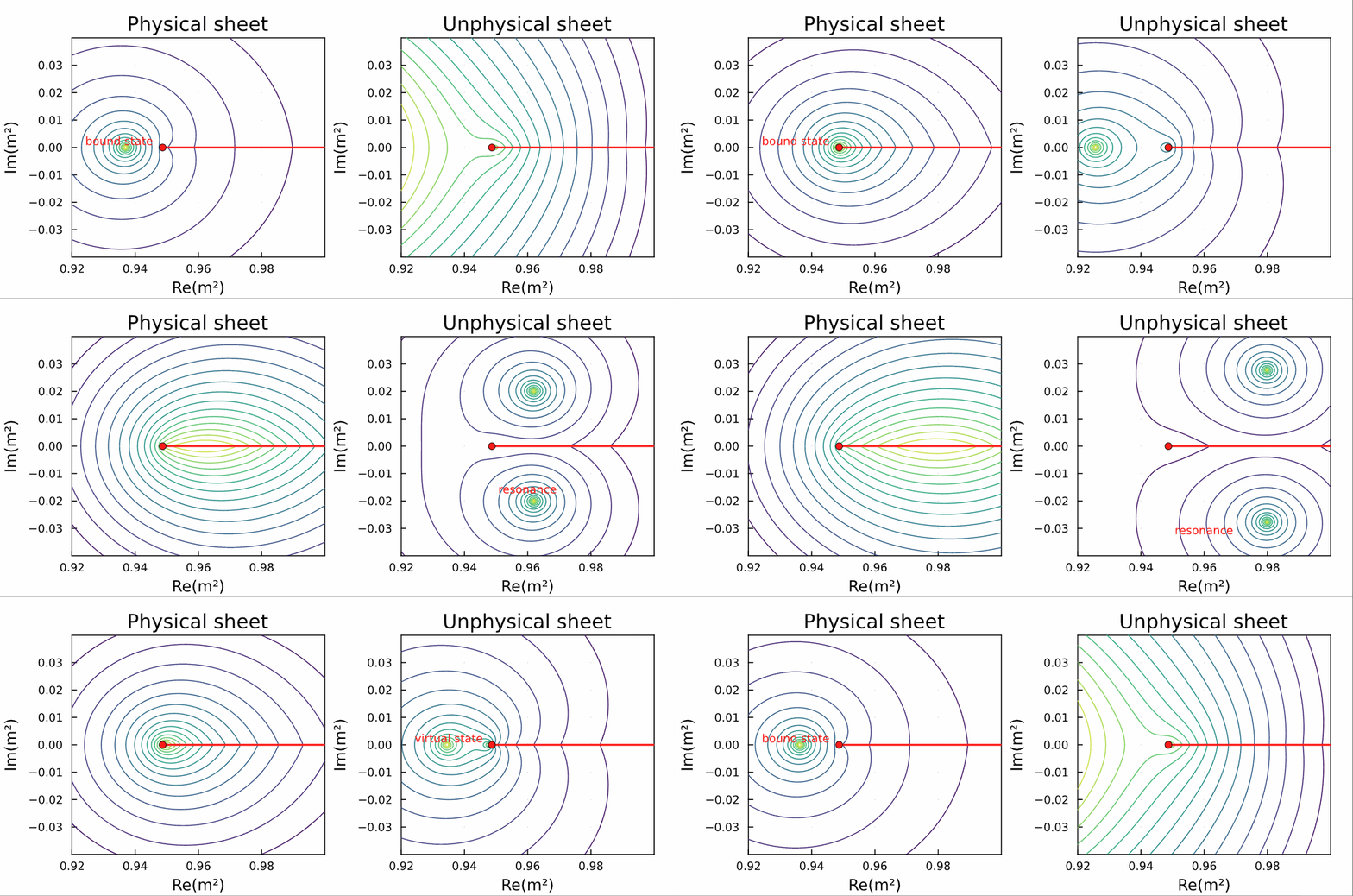
Bound → virtual → resonance: a pole can move continuously as the interaction changes.
These are different pole locations, not three unrelated kinds of constituent.
A shallow S-wave bound state has a long-distance tail:
When exceeds the interaction range, a hadron-pair description becomes especially useful.
Summary and discussion
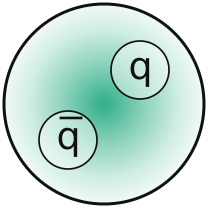
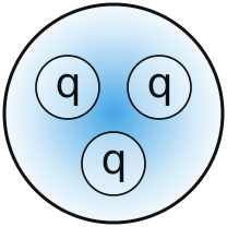
Hadron families
10 + 24 + X
Conventional hadrons probe QCD in different regimes—from light-quark dynamics to heavy-quark systems.
Exotic hadrons expand the possibilities for how QCD binds matter.
Experimental discoveries
A golden age of hadron spectroscopy: the past 15 years.
Belle / Belle II + BESIII + LHC: new forms of hadronic matter, a richer understanding of what QCD allows—and many puzzles still open.
Hadrons as resonances
S-matrix-driven physics: understand hadrons through their scattering and decay amplitudes.
Intricate mathematics of cuts, poles and Riemann sheets—with ideas reaching far beyond hadron physics.
Hadronic S-matrix → Veneziano amplitude → string theory
 123456789101112131415161718192021222324252627282930313233343536

 ⟷