Hadron Spectroscopy

Amplitude analysis: how we find hadrons in decays

Mikhail Mikhasenko · Lecture 2
AEPSHEP 2026 · Taipei
Watercolour illustration: a small world of experimental apparatus on a globe

Lecture 2 roadmap

A

The puzzle — a peak in J/ψ p

B

Kinematics — phase space, the Dalitz plot, bands and reflections

C

Spin — rotations, decay chains, the full amplitude

D

Mass dependence — line shapes and form factors

E

The full model — Λb → J/ψ p K⁻ and the pentaquarks

F

Near threshold — Tcc⁺

The puzzle

A peak is not yet a particle

A narrow peak in J/ψ p

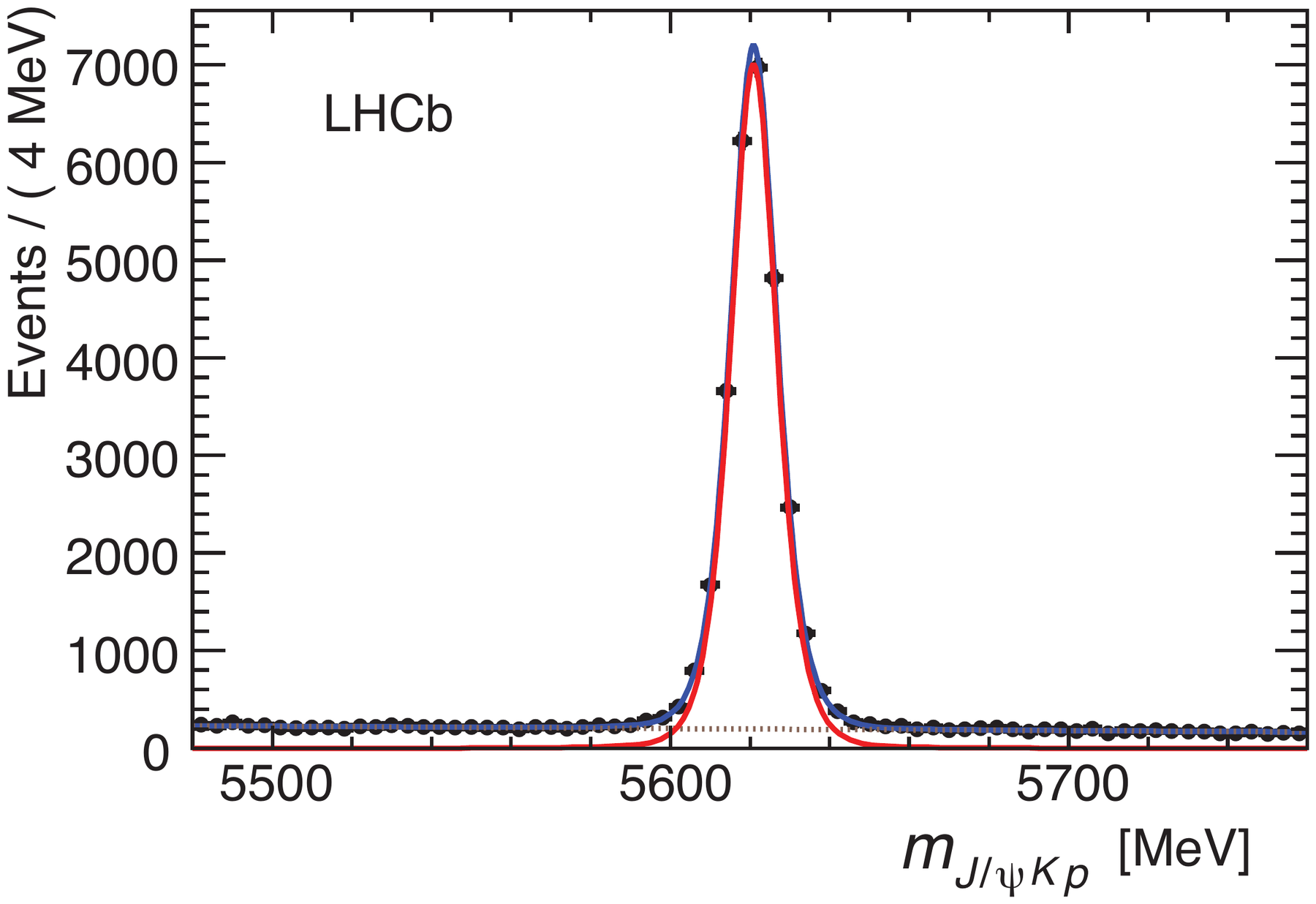
LHCb 2015: about 26 000 Λb0→J/ψpK−\Lambda_b^0\to J/\psi\,p\,K^- decays, almost no background.

The J/ψ p mass shows a narrow peak near 4.45 GeV. Phase space (red) has none.

A J/ψpJ/\psi\,p resonance would contain cc‾uudc\bar c\,uud: at least five quarks.

Is it a particle? How would we know?
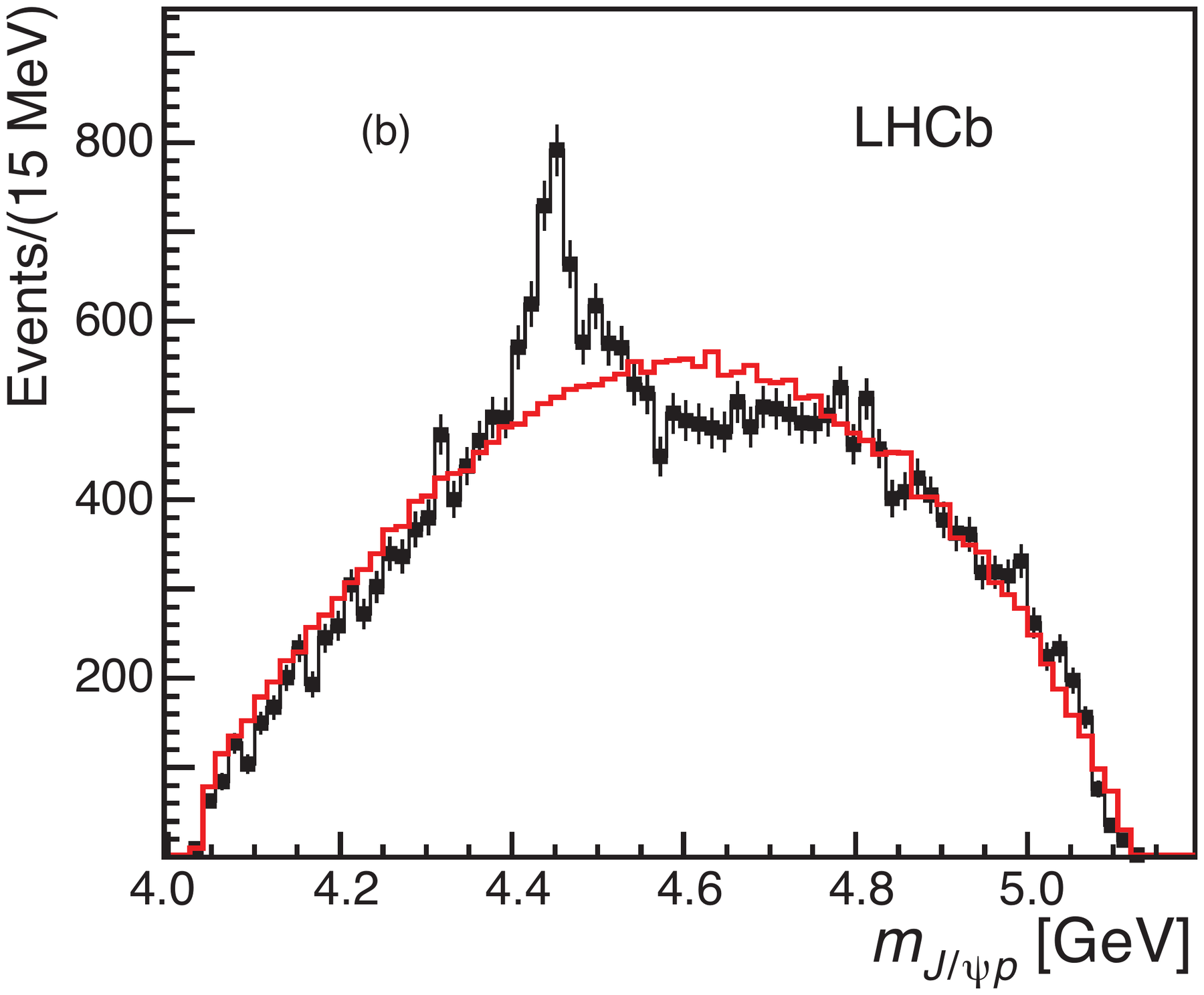
m(J/ψ p) distribution of the data compared with phase space

Reconstructing Λb → J/ψ p K⁻

A Λb is produced in a pp collision and flies a few millimetres before it decays weakly.

Four charged tracks — pp, K−K^-, μ+\mu^+, μ−\mu^- — come from one displaced vertex. The muon pair has the J/ψ mass.

Exclusive: every final-state particle is measured. Each event is a full set of four-momenta.
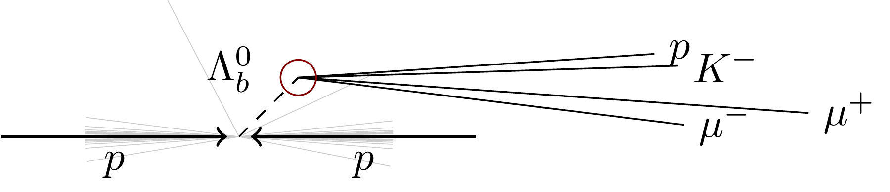
Sketch: pp collision, displaced Λb vertex with p, K⁻ and two muons Λb → J/ψ K⁻ p invariant mass: a narrow signal peak over little background

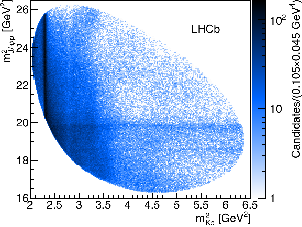
The Dalitz plot of the data

Each event is one point: two pair masses squared.

Vertical bands: Λ*→pK−\Lambda^*\to pK^- resonances, strongest the Λ(1520).

Horizontal band at m2(J/ψp)≈19.8m^2(J/\psi p)\approx 19.8 GeV²: the new structure.

The density is not uniform. Part of it is detector efficiency, the rest is physics.
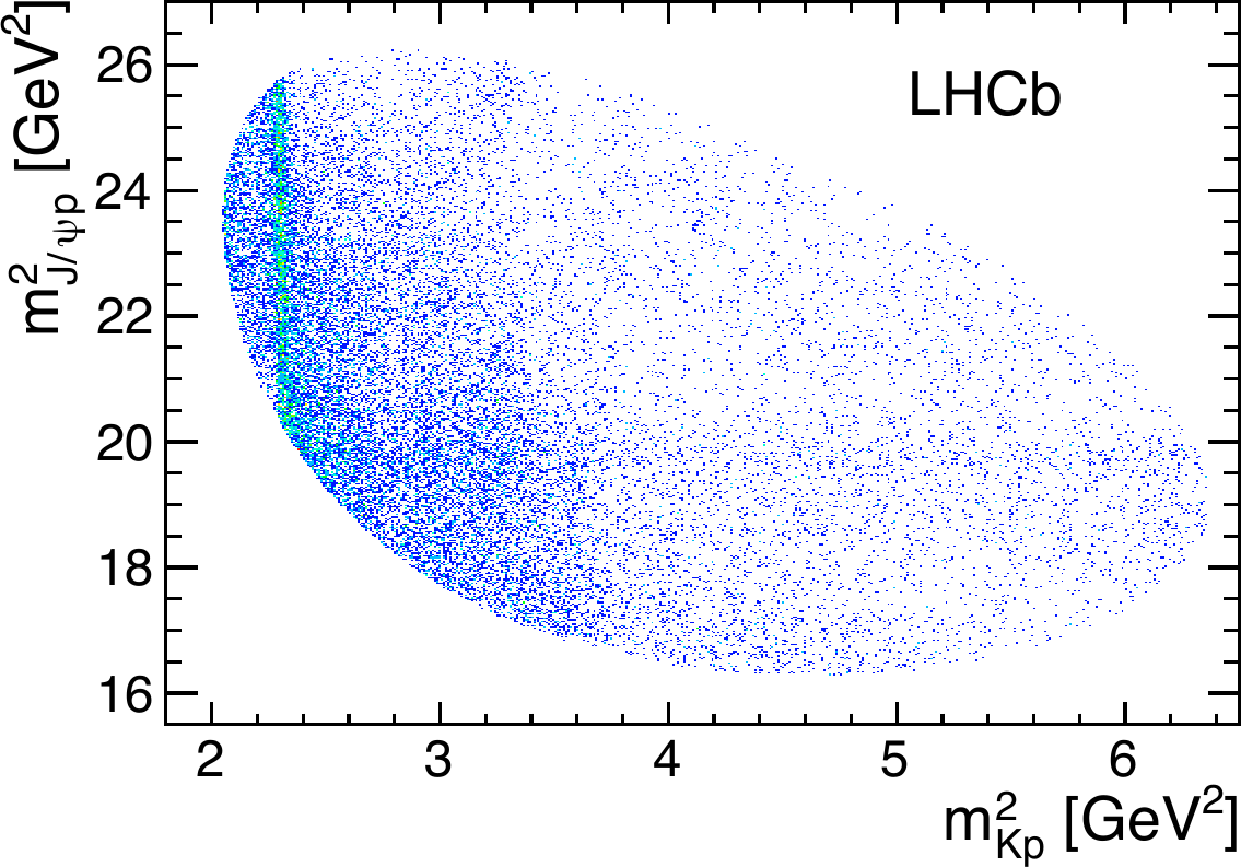
LHCb 2015 Dalitz plot of Λb → J/ψ p K⁻: m²(J/ψ p) versus m²(Kp)

Kinematics

What can vary in a three-body decay

From events to a probability

One event tells us little. Many events sample a density over the allowed momenta xx.

dN∝ϵ(x)I(x)dΦ(x) dN\;\propto\;\epsilon(x)\;I(x)\;d\Phi(x)

Lecture 1: amplitudes for the same final state interfere before squaring.

Today: build A(x) for Λb → J/ψ p K⁻, then fit it to the events.

Three factors, three questions

dΦ(x)d\Phi(x) — phase space: what kinematics allows.

I(x)=∑spins|𝒜(x)|2I(x)=\sum_{\text{spins}}|\mathcal A(x)|^2 — dynamics: what we want to learn.

ϵ(x)\epsilon(x) — detector: efficiency, known from simulation.

A structure in the data is physics only if it is in I(x)I(x).

Phase space

dΦn=d\Phi_n\;=

∏i=1nd3𝐩i(2π)32Ei\prod_{i=1}^{n}\frac{d^3\mathbf p_i}{(2\pi)^3\,2E_i}

(2π)4δ(4)(P−∑i=1npi)(2\pi)^4\,\delta^{(4)}\Big(P-\sum_{i=1}^{n}p_i\Big)

Each particle

Three momentum components 𝐩i\mathbf p_i. Dividing by 2Ei2E_i counts states the same way in every frame.

On the mass shell

Ei=mi2+|𝐩i|2E_i=\sqrt{m_i^2+|\mathbf p_i|^2}: the energy is fixed by the mass, not a new number.

Conservation

Total energy and momentum equal the parent’s: four constraints remove 4 numbers.
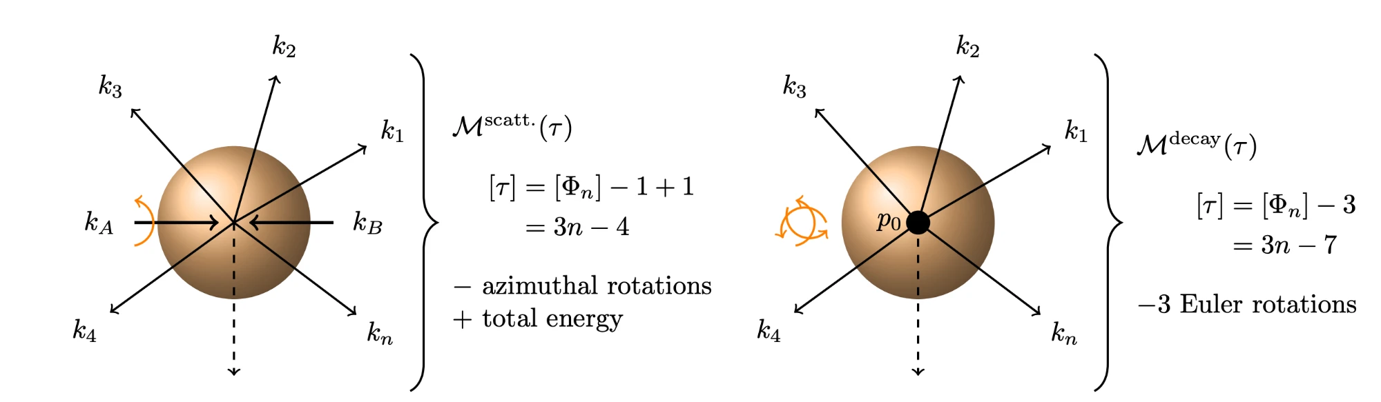
Counting the variables of a scattering and of a decay amplitude: 3n − 4, and 3n − 7 after the three Euler rotations

Two-body decay: one fixed momentum

In the parent rest frame the daughters fly back to back.

Energy conservation fixes the momentum:

q=λ(M2,m12,m22)2M q=\frac{\sqrt{\lambda(M^2,m_1^2,m_2^2)}}{2M}

Only the direction is free:

dΦ2=18π2qMdΩ4π d\Phi_2=\frac{1}{8\pi}\;\frac{2q}{M}\;\frac{d\Omega}{4\pi}

2q/M→12q/M\to1 for massless daughters; dΩ/4πd\Omega/4\pi: all directions equally likely.

λ(a,b,c) = a² + b² + c² − 2ab − 2ac − 2bc. Derivation in backup.

p K⁻ q Λ(1520) Λ(1520) → p K⁻: q = 0.243 GeV, any direction

Recursive phase space formulation

Group p and K⁻: first Λb→(pK−)J/ψ\Lambda_b\to(pK^-)\,J/\psi, then (pK−)→pK−(pK^-)\to p\,K^-.

dΦ3=dmpK22πdΦ2dΦ2 d\Phi_3=\frac{dm^2_{pK}}{2\pi}\;d\Phi_2\;d\Phi_2

An exact identity for every event: no resonance is assumed. Resonances will live in the same two steps.

Integrate the three orientation angles:
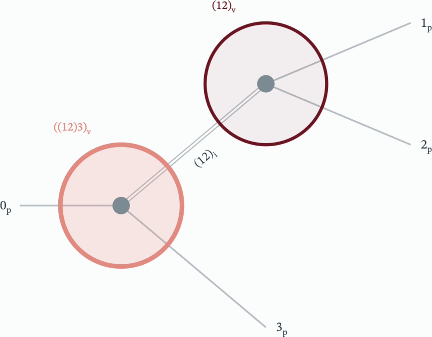
dΦ3∝dmpK2dmJ/ψp2 d\Phi_3\;\propto\;dm^2_{pK}\;dm^2_{J/\psi p}

Decay-Web-Page sketch of a decay chain: vertex ((12)3) followed by vertex (12)

H. Jonas, DEMOS, Decay-Web-Page: the chain 0 → (12) + 3, then (12) → 1 + 2.

Five numbers: shape and orientation

Three momenta: 3×3=93\times3=9 numbers.

Energy–momentum conservation removes 4.

dimΦn=3n−4=5 \dim\Phi_n=3n-4=5

Two pair masses fix the shape of the momentum triangle: they span the Dalitz plot.

Three Euler angles orient it in space.

Spin projections are labels, not extra coordinates.
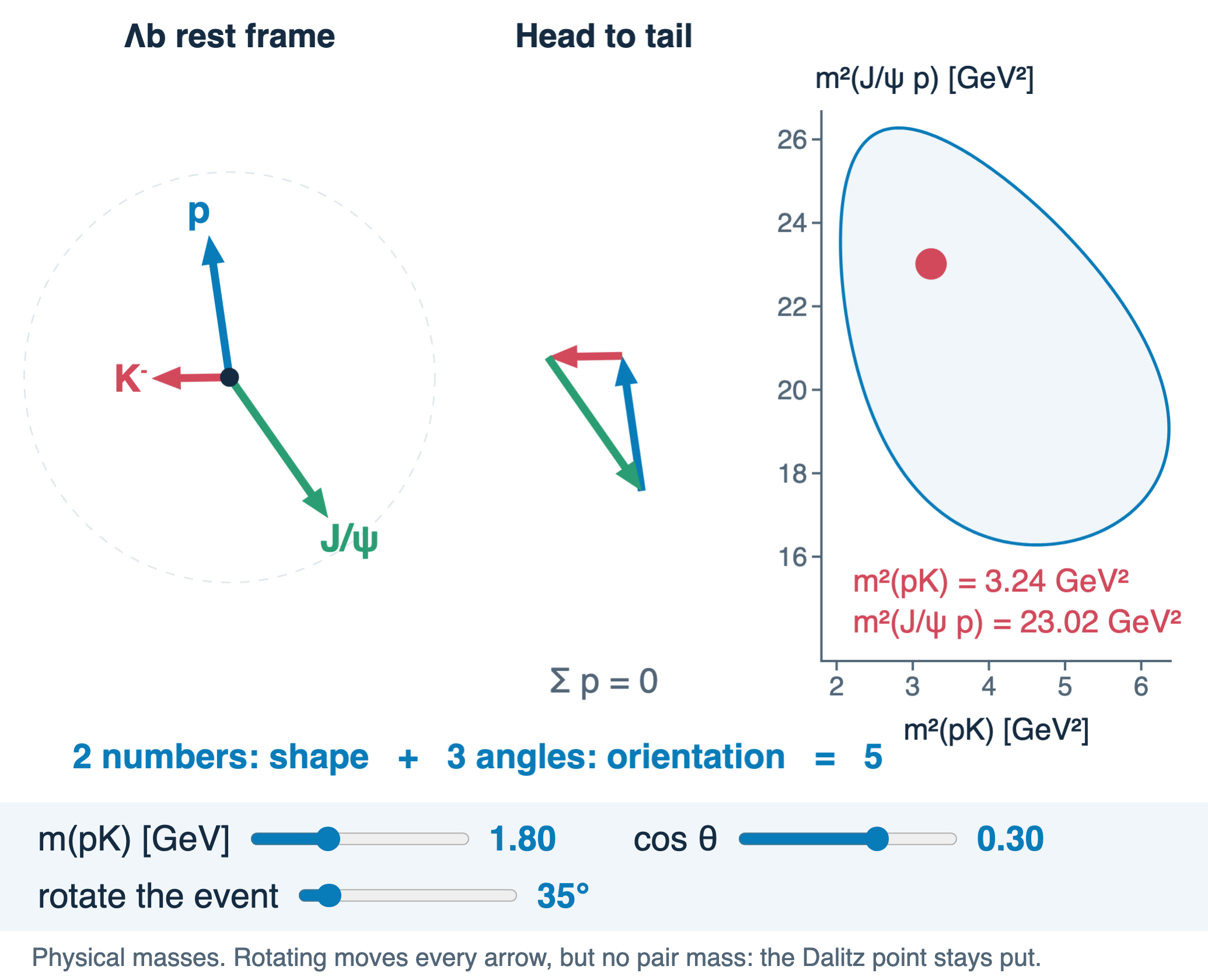
Widget: one Λb event, its momentum triangle and its Dalitz point

The phase space is flat

Phase-space events fill the plot uniformly inside the boundary.

A projection counts the height of the plot at each mass: its curved shape is pure kinematics.

In mm rather than m2m^2: dN/dm=2mdN/dm2\;dN/dm=2m\,dN/dm^2.

Any non-uniformity in the data is dynamics or detector.
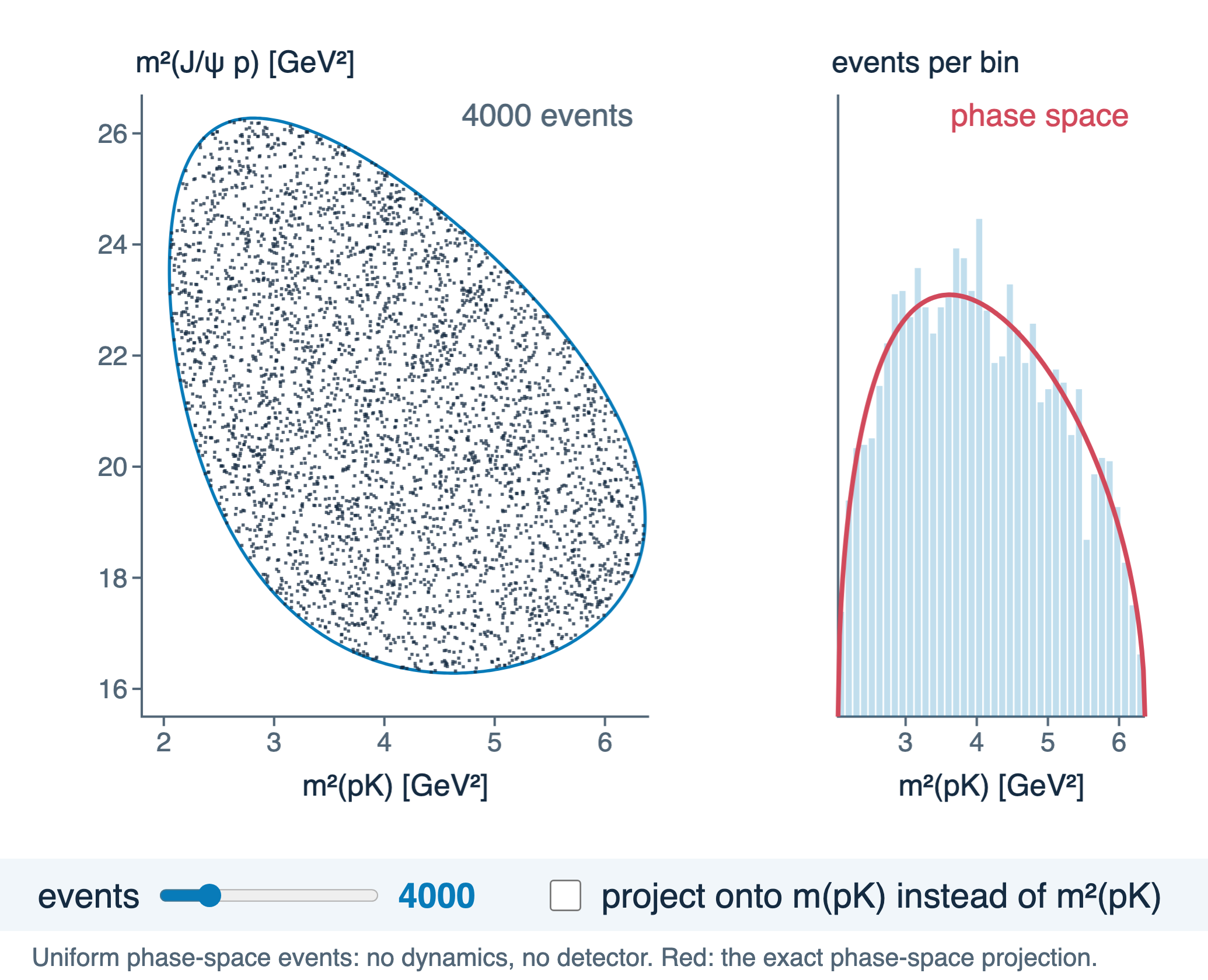
Widget: uniform phase-space events and their projection

One mass and one angle

Fix m(pK)m(pK): the event moves along a vertical slice.

The position on the slice is an angle: the proton direction in the pK rest frame.

mJ/ψp2=a+bcosθ m^2_{J/\psi p}=a+b\cos\theta

The Dalitz plot is a mass and an angle. Angular distributions sit along every band.
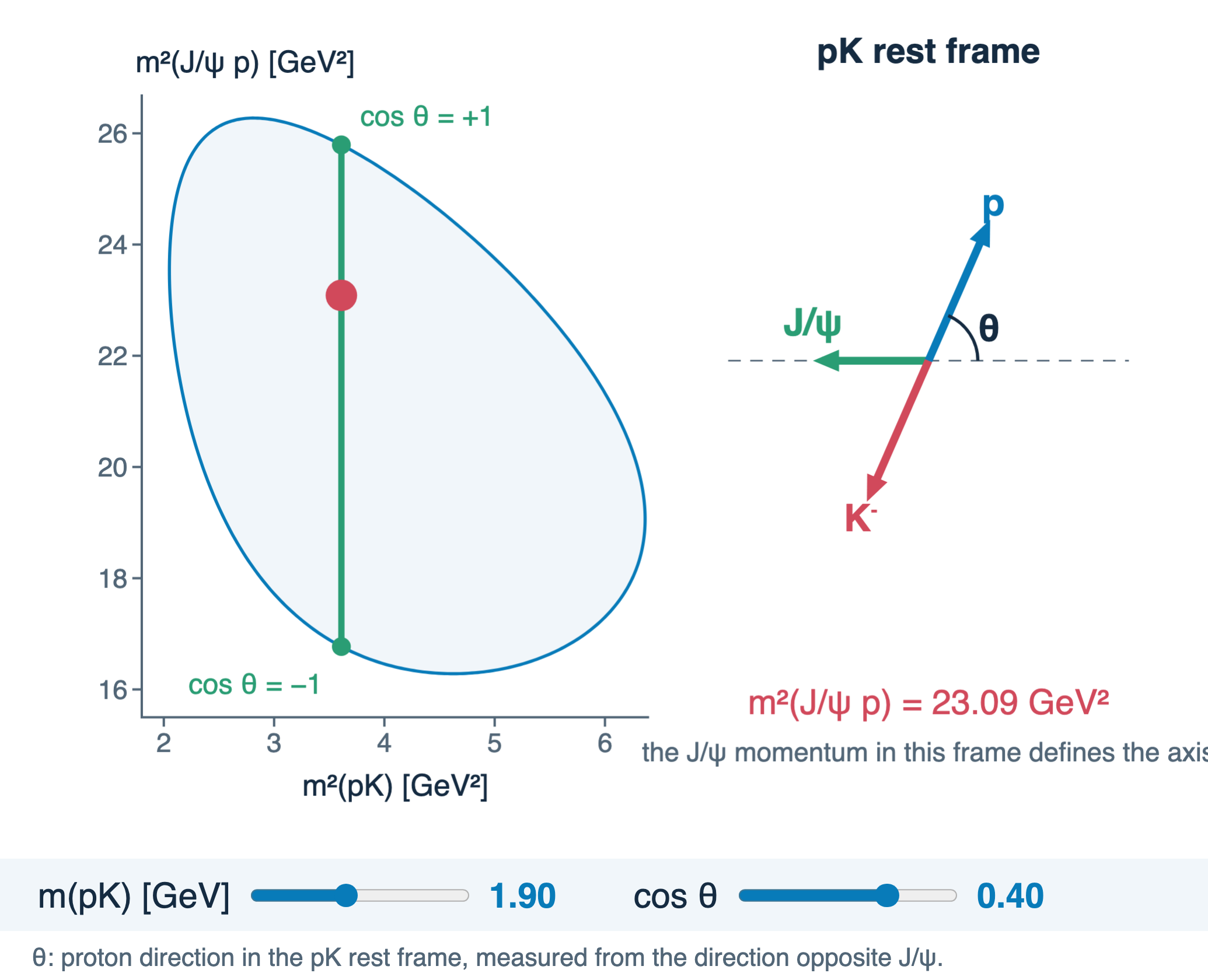
Widget: a vertical slice of the Dalitz plot and the helicity angle in the pK rest frame

Bands and reflections

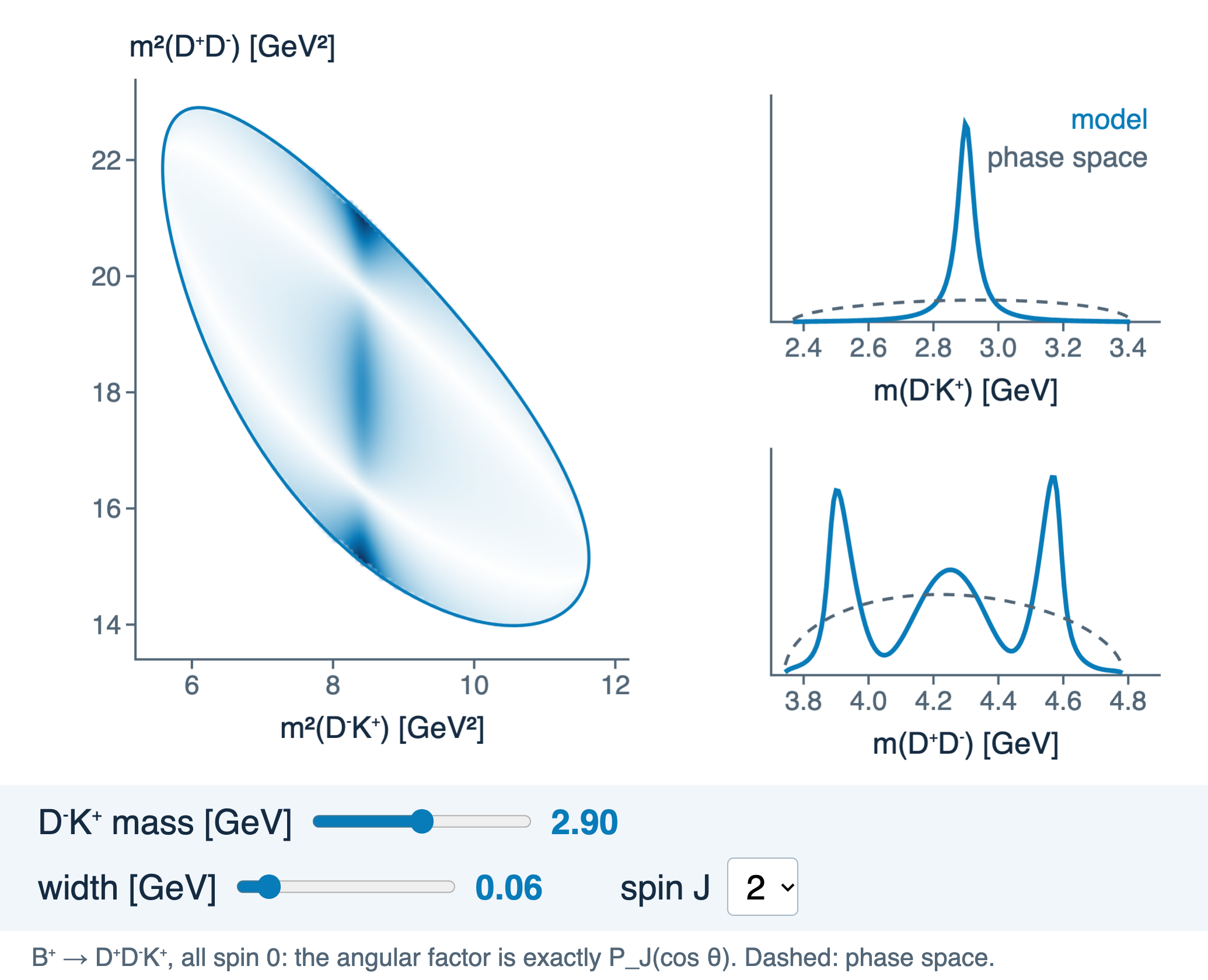
Simplest case first: B+→D+D−K+B^+\to D^+D^-K^+, all spin 0.

A resonance in D−K+D^-K^+ makes a band at fixed m(D−K+)m(D^-K^+).

Projected onto m(D+D−)m(D^+D^-), the same band gives a broad structure: a reflection. No D+D−D^+D^- resonance is needed.

Narrow peaks are hard to fake. Broad structures are easy.
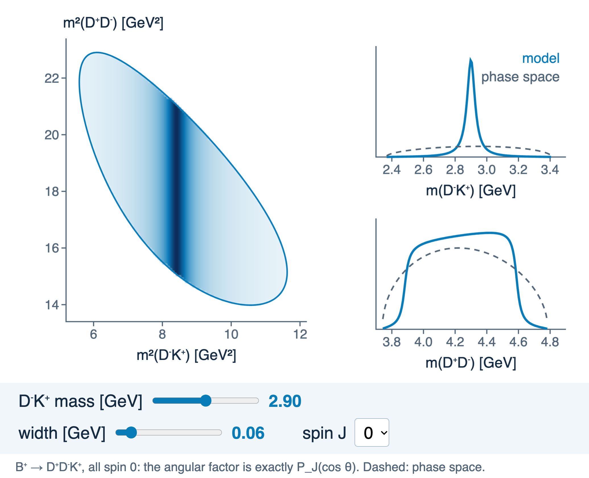
Widget: one spin-0 D⁻K⁺ band and both mass projections

Spin leaves a pattern along a band

Spin-JJ resonance → two spinless particles:

𝒜∝d00J(θ)=PJ(cosθ) \mathcal A\propto d^J_{00}(\theta)=P_J(\cos\theta)

JJ zeros along the band.

Spin also shapes the reflection: bumps in m(D+D−)m(D^+D^-) without any D+D−D^+D^- state.

Widget: a spin-2 D⁻K⁺ band with two zeros and its reflection

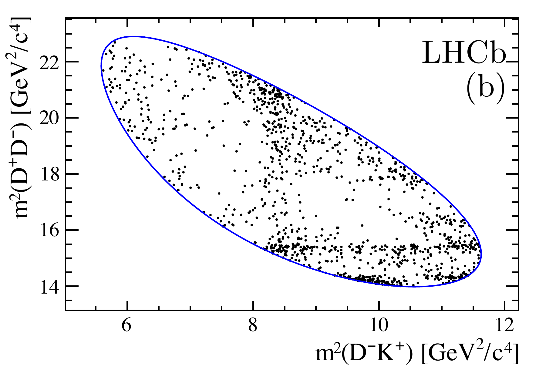
B⁺ → D⁺D⁻K⁺: the data

LHCb B⁺ → D⁺D⁻K⁺ Dalitz plot
Horizontal bands: charmonia in D⁺D⁻
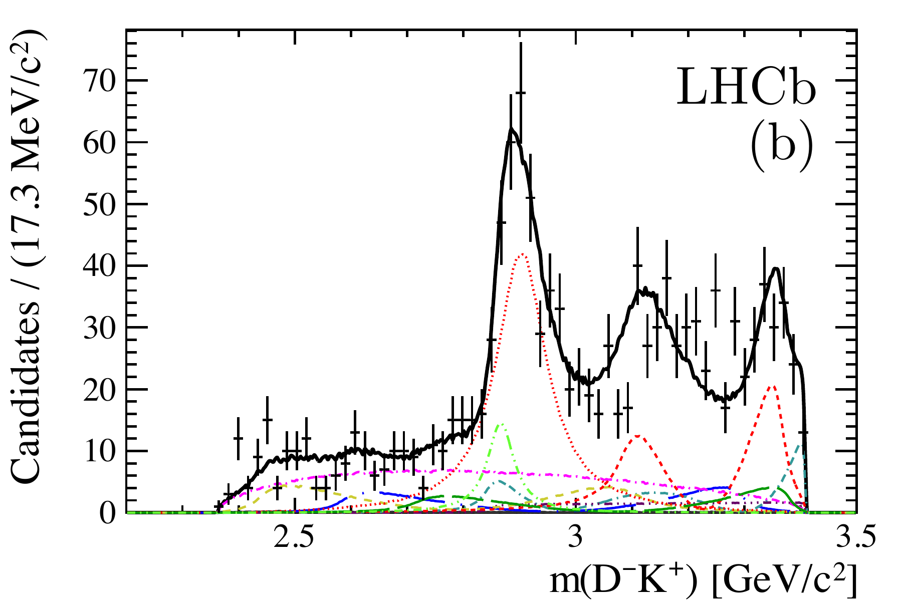
m(D⁻K⁺) projection with the amplitude fit
m(D⁻K⁺) with the full amplitude fit

The pattern along the D⁻K⁺ band, as in the widget, fixes the spin.

Charmonium bands reflect into m(D⁻K⁺), but cannot explain the peak at 2.9 GeV.

The fit needs D⁻K⁺ states with spin 0 and 1. Quark content c‾s‾ud\bar c\bar s ud: manifestly exotic.

Spin

Angular patterns, decay chains and frames

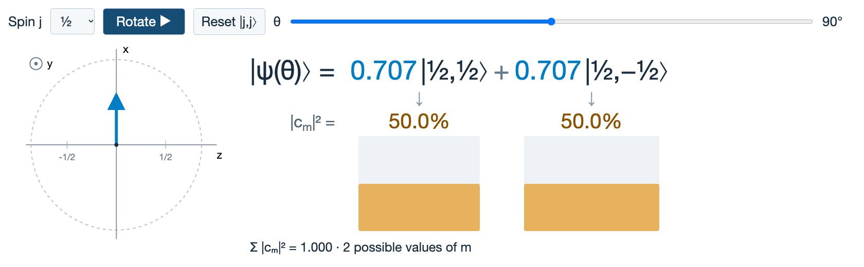
Spin rotation, revisited

Lecture 1 spin rotation widget

dm′mj(θ)d^{\,j}_{m'm}(\theta)

dm′mj(θ)=⟨j,m′|e−iθJy|j,m⟩d^{\,j}_{m'm}(\theta)=\langle j,m'|\,e^{-i\theta J_y}\,|j,m\rangle: the Wigner d-functions are the coefficients above. Amplitudes, with signs.

With three Euler angles, Dm′mj(α,β,γ)=e−im′αdm′mj(β)e−imγ\;D^{j}_{m'm}(\alpha,\beta,\gamma)=e^{-im'\alpha}\,d^{\,j}_{m'm}(\beta)\,e^{-im\gamma}.

One decay vertex

For A(J,m)→1+2A(J,m)\to 1+2 with helicities λ1,λ2\lambda_1,\lambda_2:

𝒜m;λ1λ2=Dm,λ1−λ2J*(ϕ,θ,0)⏟rotations: fixedHλ1λ2⏟fitted \mathcal A_{m;\lambda_1\lambda_2}=\underbrace{D^{J*}_{m,\lambda_1-\lambda_2}(\phi,\theta,0)}_{\text{rotations: fixed}}\;\underbrace{H_{\lambda_1\lambda_2}}_{\text{fitted}}

Helicity: spin along the particle’s momentum.

The angles are those of particle 1 in the rest frame of A.

How many couplings H?

One per allowed (L,S)(L,S) combination.

Strong Λ(1520)[32−]→pK−\Lambda(1520)\,[\tfrac32^-]\to p\,K^-: parity allows only L=2L=2 → 1 coupling.

Weak Λb→Λ*J/ψ\Lambda_b\to\Lambda^*J/\psi: no parity constraint → 4 couplings (J=12J=\tfrac12) or 6 (J≥32J\ge\tfrac32).

Each is a complex number to fit.

A decay chain

Λb→Λ*J/ψ\Lambda_b\to\Lambda^*J/\psi, then Λ*→pK−\Lambda^*\to pK^-:

𝒜Λ*=∑ν𝒜νΛb→Λ*ψBW(mpK2)𝒜νΛ*→pK \mathcal A^{\Lambda^*}=\sum_{\nu}\;\mathcal A^{\Lambda_b\to\Lambda^*\psi}_{\nu}\;\,\mathrm{BW}(m^2_{pK})\;\,\mathcal A^{\Lambda^*\to pK}_{\nu}

Two vertices, each in its own rest frame, joined by a propagator.

The Λ* helicity ν\nu is not observed and is internal: sum the amplitudes.
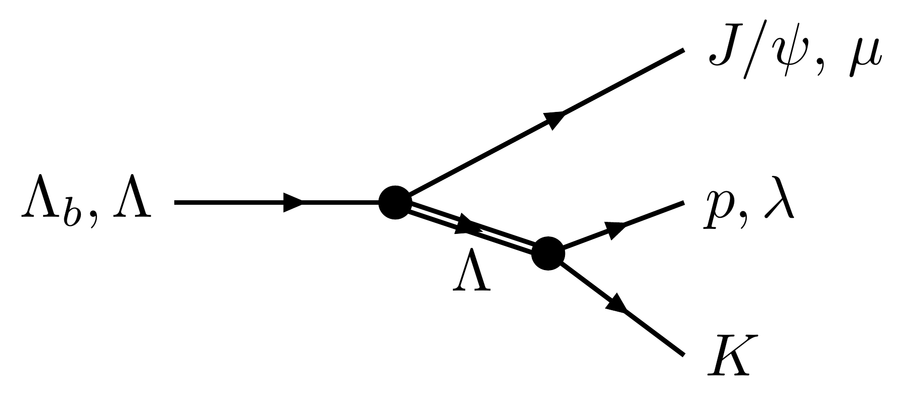
Diagram: Λb → Λ* J/ψ, Λ* → p K

Labels Λ, μ, λ beside the external lines are spin projections; the internal Λ is the Λ*.

Two chains, one final state
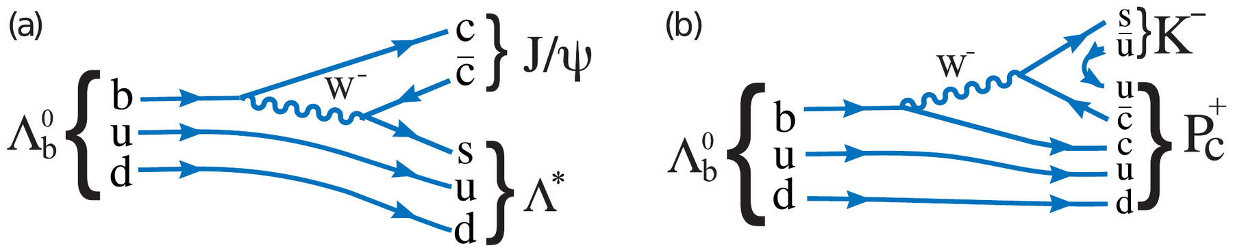
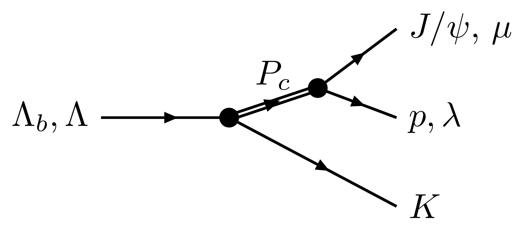
Quark-line diagrams: Λb → J/ψ Λ*, and Λb → Pc⁺ K⁻

Λ* chain: b→cc‾sb\to c\bar c s; the ss quark forms an excited Λ* with udud.

Pc chain: the cc‾c\bar c pair stays with uuduud and recoils against K−K^-.

Same particles, same momenta: the amplitudes add, then we square.

The full amplitude

One decay chain: two vertices and a propagator.

DJ0*(Ω0)D^{J_0*}(\Omega_0)

angles

FF(m0;mR,mk)FF(m_0;\,m_R,\,m_k)

form factor

vertex Λb → R k

R(mR2)R(m_R^2)

line shape

R propagates

DJR*(ΩR)D^{J_R*}(\Omega_R)

angles

FF(mR;mi,mj)FF(m_R;\,m_i,\,m_j)

form factor

vertex R → i j

Λ* chain diagram: Λb → Λ* J/ψ, Λ* → p K
Σ over Λ* states
Pc chain diagram: Λb → Pc K, Pc → J/ψ p
Σ over Pc states

𝒜λ=∑chains kckAλ(k)I=∑λ|𝒜λ|2 \mathcal A_\lambda=\sum_{\text{chains }k}\,c_k\,A^{(k)}_\lambda\qquad\qquad I=\sum_{\lambda}\big|\mathcal A_\lambda\big|^2

Rotations: fixed by spin (this section)

Mass dependence: model choices (next section)

ckc_k: complex couplings, fitted

Coherent over chains, incoherent over unobserved spins. Pc chains also need the spin alignment d(ζ) (backup).

Frames, live

Start in the laboratory: the Λb flies.

Rotate, then boost, into the Λb rest frame.

Repeat for the pK⁻ pair: its rest frame, with the z axis along its flight direction.

Every angle in the amplitude is measured in such a frame.
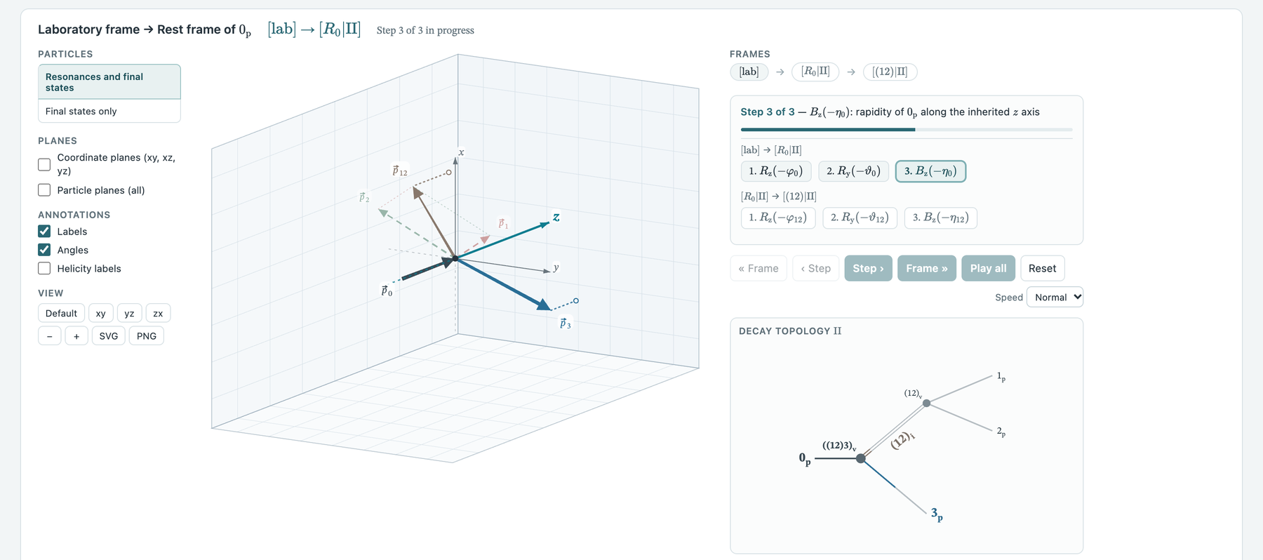
Decay-Web-Page Dynamic view: three-dimensional momenta and the steps from the laboratory to the rest frames

Mass dependence

Line shapes and vertex form factors

The resonance line shape

R(mR2)R(m_R^2): how the resonance propagates. The typical construction is a Breit–Wigner with a running width:

R(σ)=1mR2−σ−imRΓ(σ) R(\sigma)=\frac{1}{m_R^2-\sigma-i\,m_R\,\Gamma(\sigma)}

Γ(σ)=ΓRqqRmRσFFL2(σ) \Gamma(\sigma)=\Gamma_R\,\frac{q}{q_R}\,\frac{m_R}{\sqrt\sigma}\,FF_L^2(\sigma)

A peak in |R|2|R|^2, and a phase that rises through 90° (Lecture 1). The width carries the decay form factor (next slide).
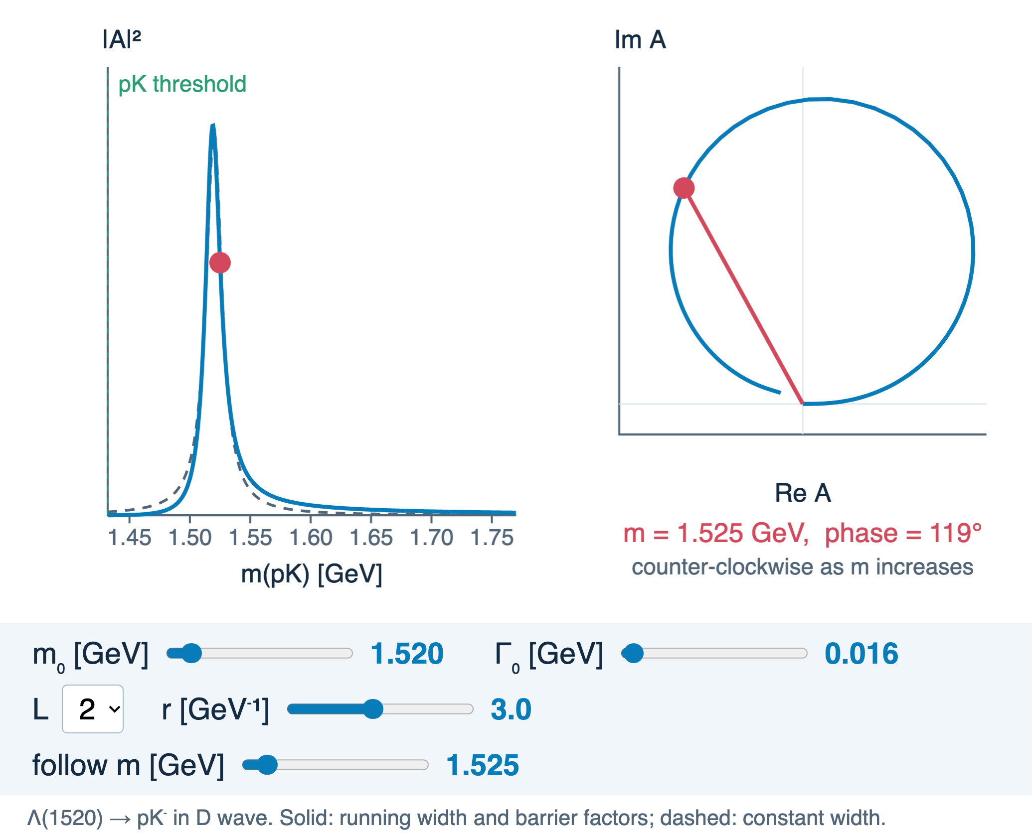
Widget: Λ(1520) line shape and its path in the complex plane

Form factors

FF(m0;m1,m2)FF(m_0;\,m_1,m_2): the vertex where m0→m1+m2m_0\to m_1+m_2, with breakup momentum qq.

FFL=(qq0)LBL(qr)BL(q0r) FF_L=\Big(\frac{q}{q_0}\Big)^{L}\,\frac{B_L(qr)}{B_L(q_0r)}

qLq^L: the angular-momentum barrier. Partial wave LL is suppressed near threshold.

Blatt–Weisskopf BLB_L: stops the growth for q≳1/rq\gtrsim1/r, with r≈r\approx 1.5–5 GeV⁻¹ (0.3–1 fm).

B₁ = 1/√(1+z²), B₂ = 1/√(9+3z²+z⁴), z = qr. Two vertices, two form factors: production uses p, decay uses q.
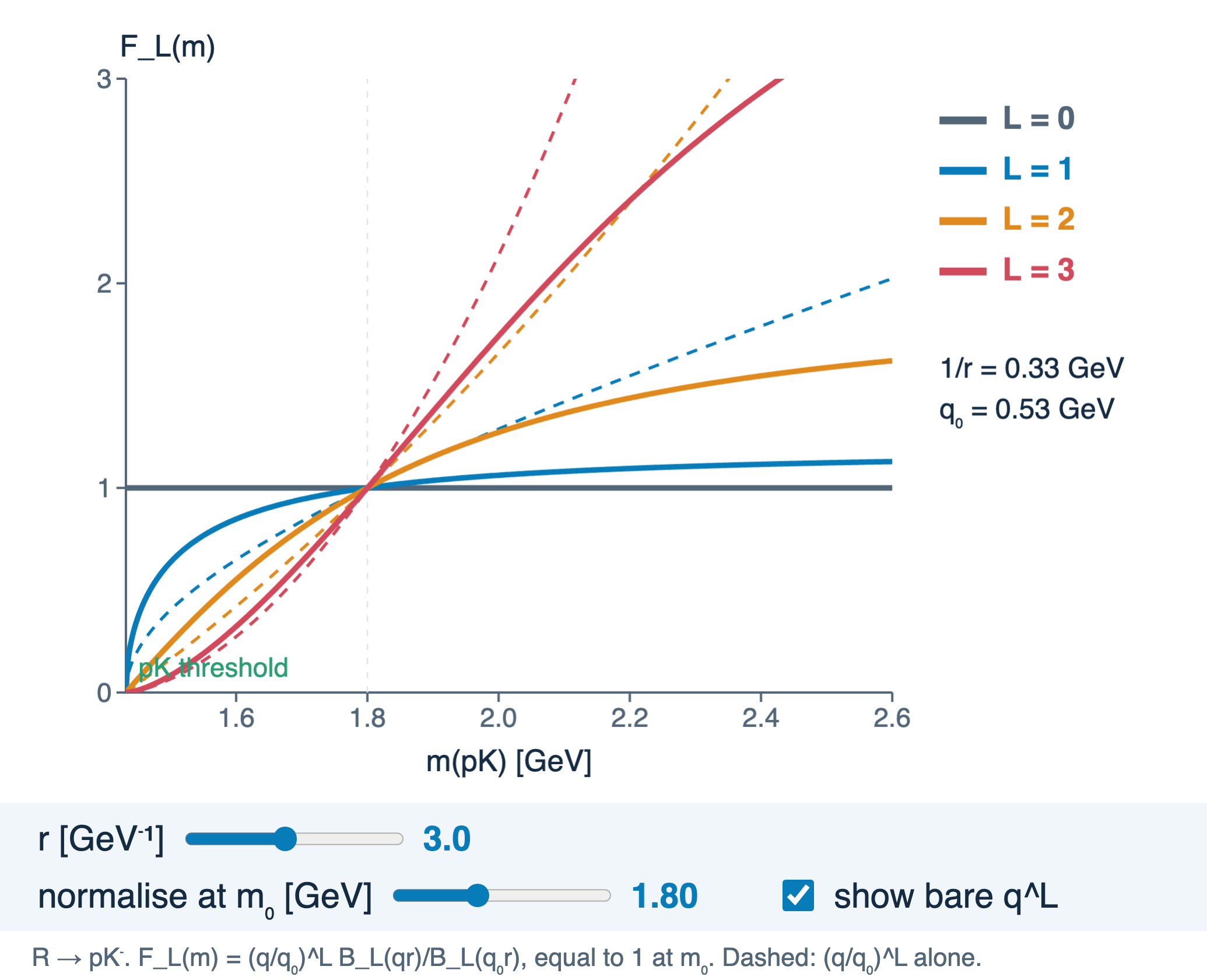
Widget: vertex form factor versus m(pK) for L = 0 to 3

The full model: Λb → J/ψ p K⁻

Spin, interference and the pentaquarks

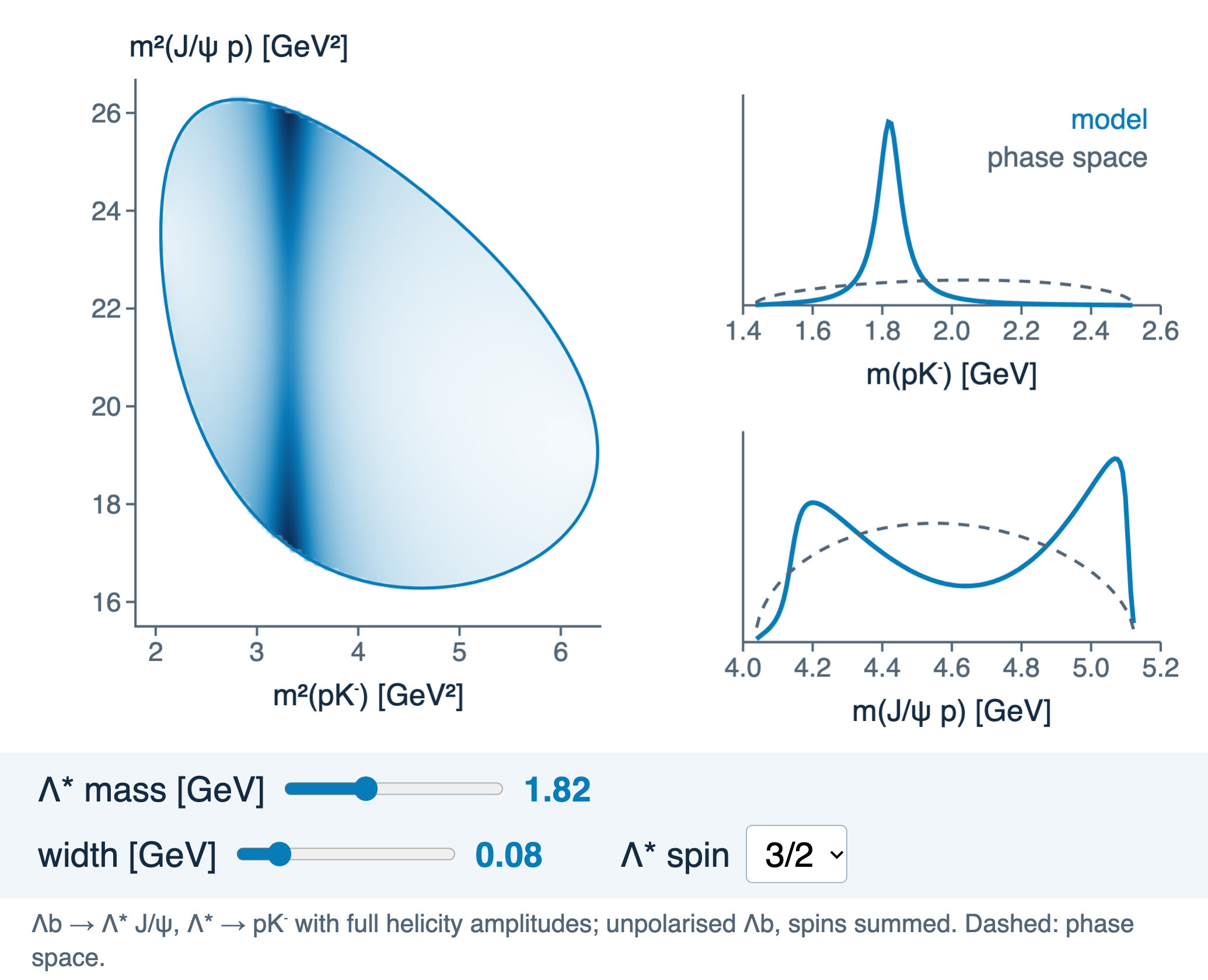
With a proton, the zeros fill in

Back to Λ*→pK−\Lambda^*\to pK^-: the proton has two helicities, ±12\pm\tfrac12.

Its spin is not measured: add |A|2|A|^2 for both.

Each term has zeros; the sum does not. For J=32J=\tfrac32:

|d12123/2|2+|d12,−123/2|2∝1+3cos2θ |d^{3/2}_{\frac12\frac12}|^2+|d^{3/2}_{\frac12,-\frac12}|^2\propto 1+3\cos^2\theta

Spin is still visible, but less sharply. LHCb also used the J/ψ → μ⁺μ⁻ angles.
Widget: a spin-3/2 Λ* band in Λb → J/ψ p K⁻ without zeros

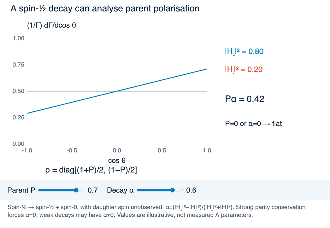
Unpolarised and polarised parents

The parent’s spin states form an ensemble, described by a density matrix:

I(x)=∑final spins∑m,m′ρmm′𝒜m𝒜m′* I(x)=\sum_{\text{final spins}}\;\sum_{m,m'}\rho_{mm'}\,\mathcal A_m\mathcal A^*_{m'}

Unpolarised (ρ∝1\rho\propto 1): no preferred direction. Integrate the orientation; the Dalitz variables remain.

Polarised: the production angles — the orientation of the decay relative to the polarisation axis — become anisotropic: 1+αPcosθ1+\alpha P\cos\theta.

Λb at LHCb: P compatible with zero. Λc⁺ → pK⁻π⁺ as a polarimeter: paper, website.
Widget: spin-1/2 decay angular distribution for parent polarisation P and analysing power α

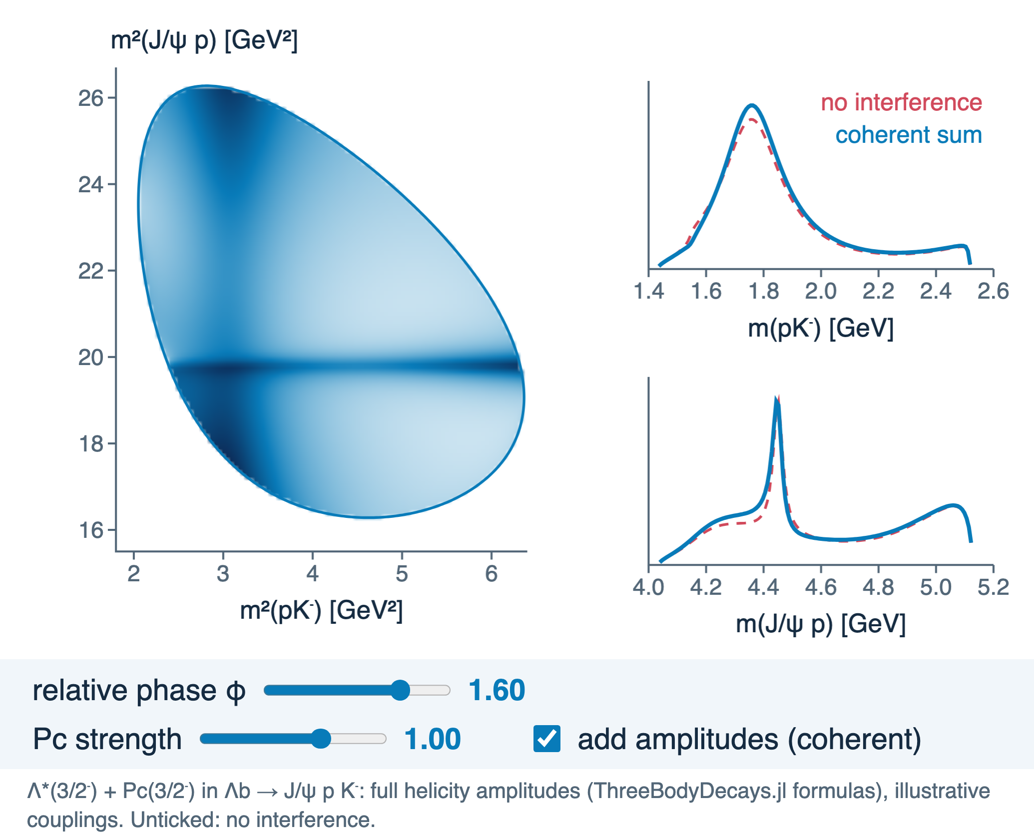
Interference reshapes the plot

|A1+A2|2=|A1|2+|A2|2+2ReA1A2* |A_1+A_2|^2=|A_1|^2+|A_2|^2+2\,\mathrm{Re}\,A_1A_2^*

The cross term follows the relative phase: the Dalitz pattern and the Pc line shape change.

Summing over spins dilutes it, but does not remove it.

The projection alone cannot tell. The fit measures the phase.
Widget: a Λ* band and a Pc band interfering with relative phase 1.6 rad

Λ* states alone fail

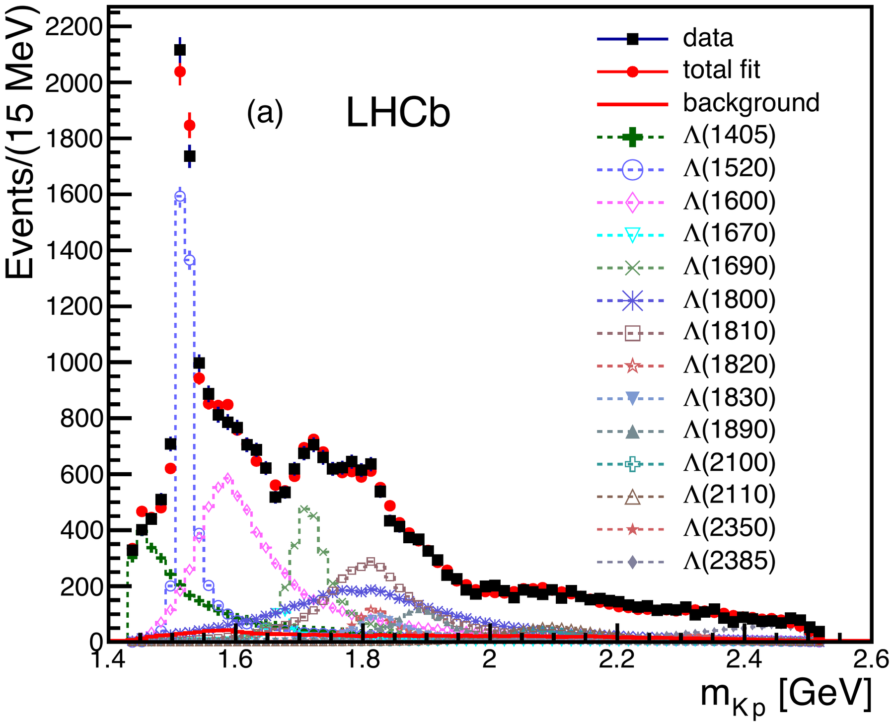
m(Kp) projection of the Λ*-only fit
m(Kp): the Λ* states describe their own channel
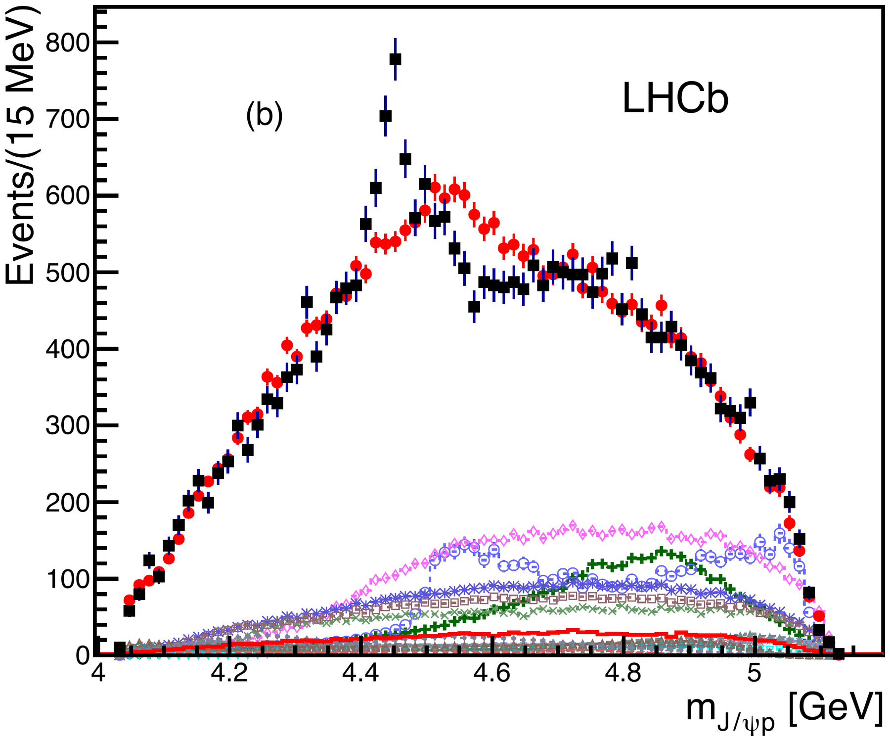
m(J/ψ p) projection of the Λ*-only fit, missing the peak
m(J/ψ p): the peak is missed

Fit with all 14 Λ* states and every allowed coupling.

The reflections are included, with all interference.

The narrow structure near 4.45 GeV is still not described.

Adding Pc states

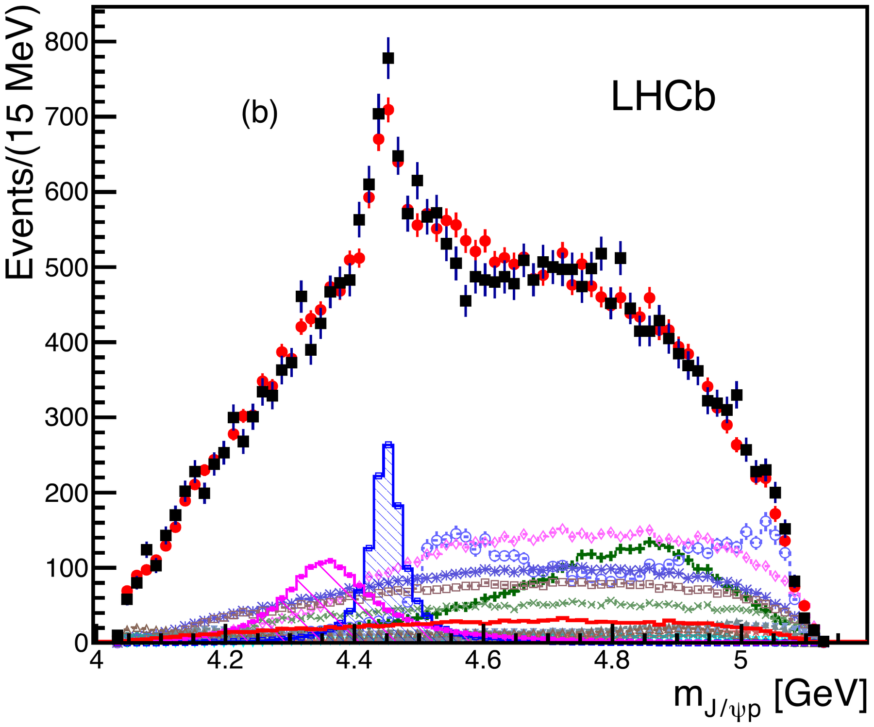
Add two J/ψ p states to the Λ* model: now the data are described.

A narrow Pc(4450)⁺ (Γ ≈ 40 MeV) and a broad Pc(4380)⁺ (Γ ≈ 200 MeV). Stat. significance: 12σ and 9σ.

Opposite parities; best spins 32\tfrac32 and 52\tfrac52, from the decay angles.

There was more to discover…
m(J/ψ p) fit with two Pc states

2019: more data, a new picture

LHCb 2019 Dalitz plot
Nine times more Λb decays
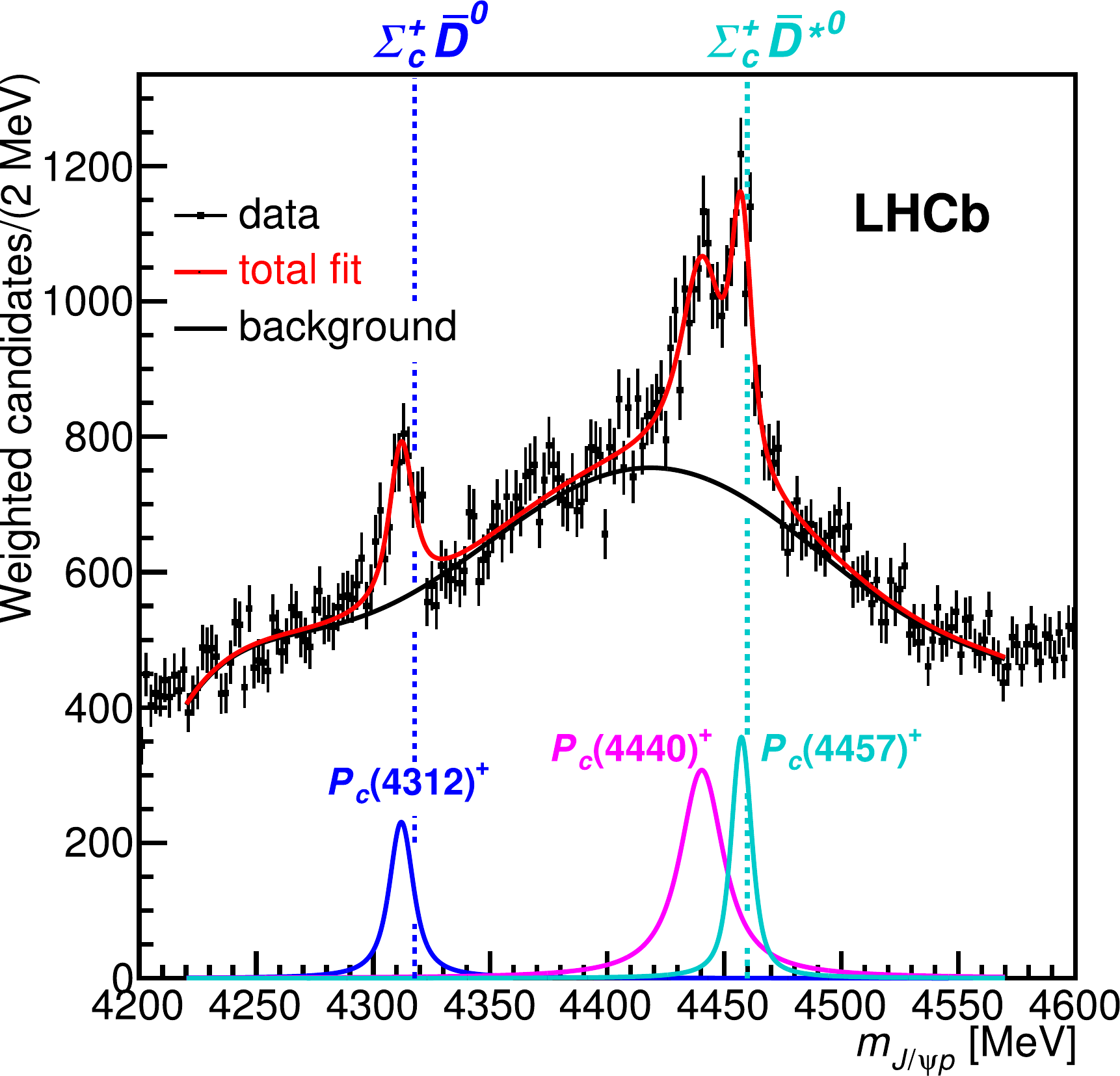
m(J/ψ p) with three narrow Pc peaks
Three narrow peaks in m(J/ψ p)

The 4450 structure splits into Pc(4440)⁺ and Pc(4457)⁺. A new Pc(4312)⁺ appears.

A fit of the mass projection: spins are not determined; the broad Pc(4380)⁺ neither confirmed nor excluded.

Pentaquarks: measured and interpreted

Measured

Three narrow peaks: Pc(4312)⁺, Pc(4440)⁺, Pc(4457)⁺, widths 6–20 MeV.

Each sits 2–20 MeV below a Σc+D‾0\Sigma_c^+\bar D^{0} or Σc+D‾*0\Sigma_c^+\bar D^{*0} threshold. Spins not yet determined.

Interpreted

ΣcD‾(*)\Sigma_c\bar D^{(*)} molecules give this pattern naturally (Lecture 1). Compact pentaquarks and threshold effects are also discussed.

Deciding needs spins, partner states and poles — from amplitude analyses.
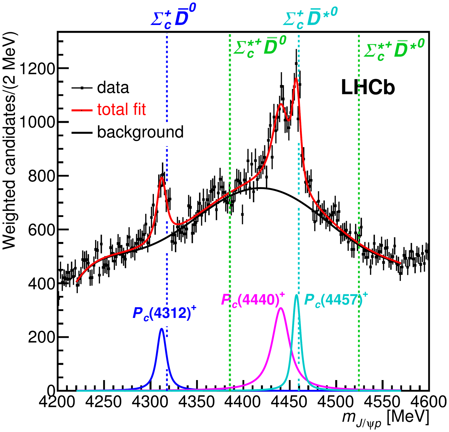
m(J/ψ p) with three narrow Pc peaks and the Σc D̄ and Σc D̄* thresholds

2027: the full amplitude analysis

The full amplitude analysis of the Run 1 + 2 sample is about to be finished.

It is very complicated.

Why it takes so long

High statistics: small effects become significant; the model must describe them all.

Coupled-channel dynamics: narrow states at the Σc D̄(*) thresholds need more than Breit–Wigners.

Fixes in the formalism: interference between chains needs consistent spin alignment.

Tools for amplitude models

DecaySelector: declare the particles and their JPJ^P; it lists the three decay topologies, collects the resonances in each pair, and counts the complete decay chains.

Decay-Web-Page: frames, rotations and the amplitude of each chain.

ThreeBodyDecays.jl: the amplitudes used in today’s widgets.
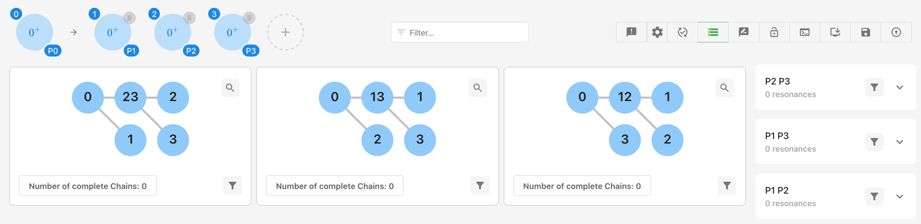
DecaySelector: particles with spin-parity, the three decay topologies and resonance lists per pair

Near threshold: Tcc⁺

When a Breit–Wigner is not enough

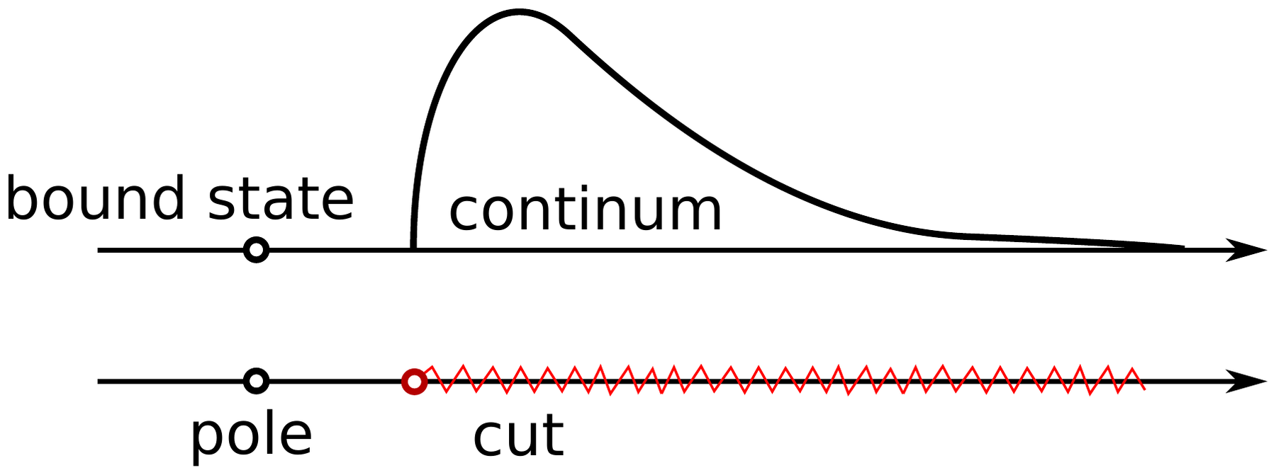
A bound state below threshold

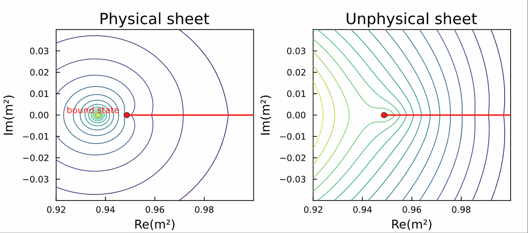
Bound state as a pole below the threshold, continuum as a cut above it
Bound state: a pole below the continuum
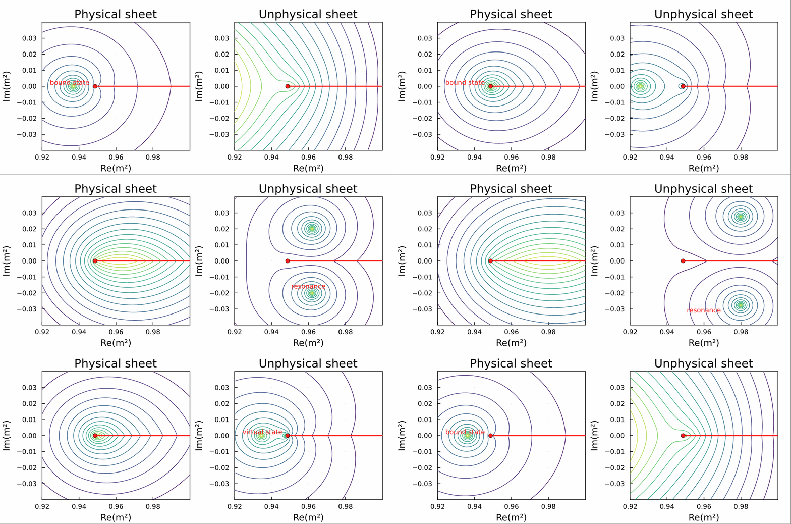
Animation of a pole moving from bound to virtual to resonance as the interaction changesFirst frame of the animation: a bound-state pole on the physical sheet
Weaker attraction: the pole moves (Lecture 1)

Below threshold, a bound state is a pole of the amplitude. Above it, free D*DD^*D pairs form the continuum: a cut.

The weaker the binding, the closer the pole to the threshold; then it becomes virtual.

A shallow bound state is large: ψ∝e−κr/r\psi\propto e^{-\kappa r}/r, κ=2μB\kappa=\sqrt{2\mu B}. For Tcc+T_{cc}^+, B≈0.36B\approx0.36 MeV gives 1/κ≈7.51/\kappa\approx7.5 fm.

The Tcc⁺ decay amplitude

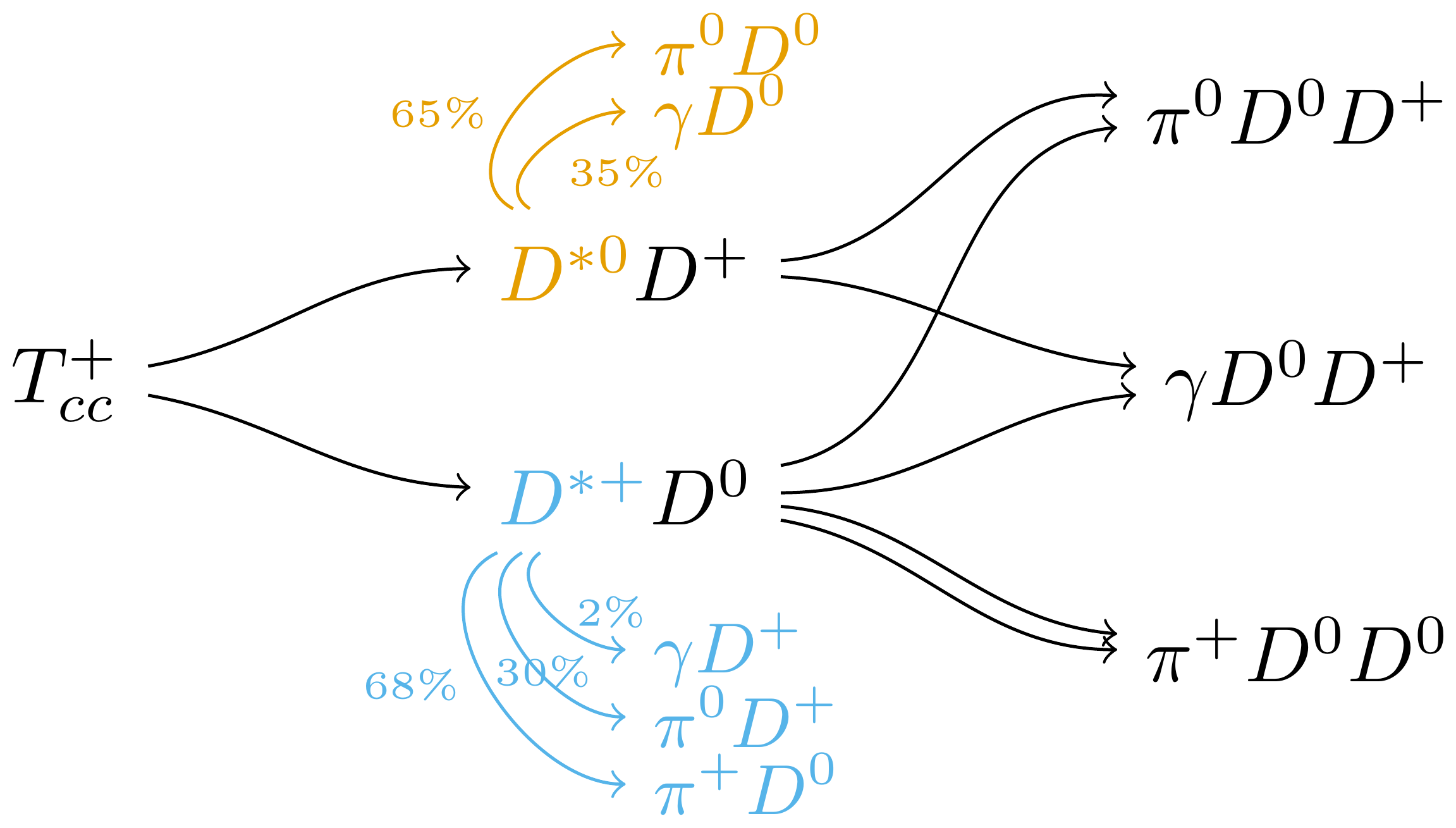
Tcc⁺ decays to D*⁺D⁰ and D*⁰D⁺; each D* decays to Dπ or Dγ, giving π⁺D⁰D⁰, π⁰D⁰D⁺ and γD⁰D⁺
Two D*D channels, three final states
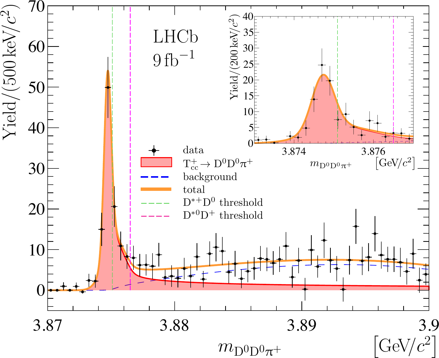
LHCb Tcc⁺ peak in D⁰D⁰π⁺ with the unitarised model fit
The unitarised model fit to D⁰D⁰π⁺

JP=1+J^P=1^+: S-wave decay to D*DD^*D. An isoscalar: equal couplings to D*+D0D^{*+}D^0 and D*0D+D^{*0}D^+.

The model is unitary: the D*D^* width and all three-body channels enter the line shape. Two parameters: peak position and coupling.

Pole: δm=−360±40\delta m=-360\pm40 keV, Γ≈48\Gamma\approx48 keV, below the D*+D0D^{*+}D^0 threshold. A constant-width Breit–Wigner misses the threshold.

Tcc and Tbb: experiment and lattice
Experiment: Tcc⁺ in D⁰D⁰π⁺
Experiment: Tcc⁺, barely bound
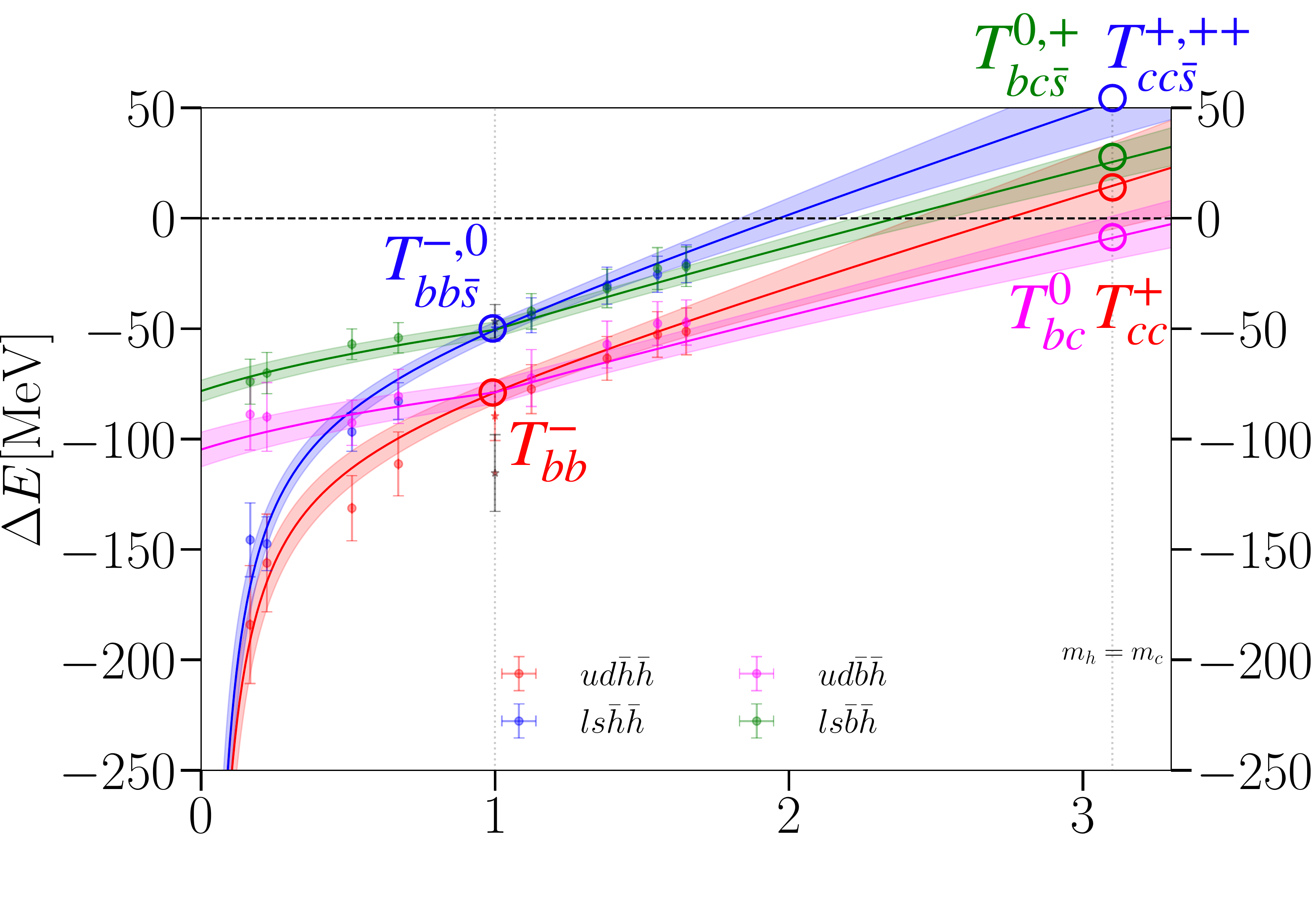
Lattice binding energies of doubly heavy 1⁺ tetraquarks versus the heavy-mass ratiorh = mb / mh
Lattice QCD: binding versus heavy-quark mass

Lattice QCD at mπ≈300m_\pi\approx 300 MeV: binding energy versus heavy-quark mass; bottom at rh=1r_h=1, charm at rh≈3r_h\approx3.

Heavier quarks bind deeper: TbbT_{bb} predicted far below threshold, stable against strong decay.

At the charm mass the lattice point is near threshold; the measured TccT_{cc} is 0.36 MeV below. TbcT_{bc} has a good chance to be discovered at the LHC.

What we have discussed

Kinematics

Five numbers per three-body event: two for the shape (the Dalitz plot), three for the orientation.

Phase space is flat; bands, reflections and spin zeros are dynamics.

Spin

Each vertex: rotation × coupling. Chains with the same final state add as amplitudes.

Mass dependence

Line shapes and form factors are model choices, tested by the fit.

Two examples: narrow tetraquarks and pentaquarks

A peak, then a model of the whole decay. Λ* states alone fail; Pc states are needed. Their nature is still open.

Tcc⁺: a narrow peak just below the D*D threshold, where a Breit–Wigner is not enough.

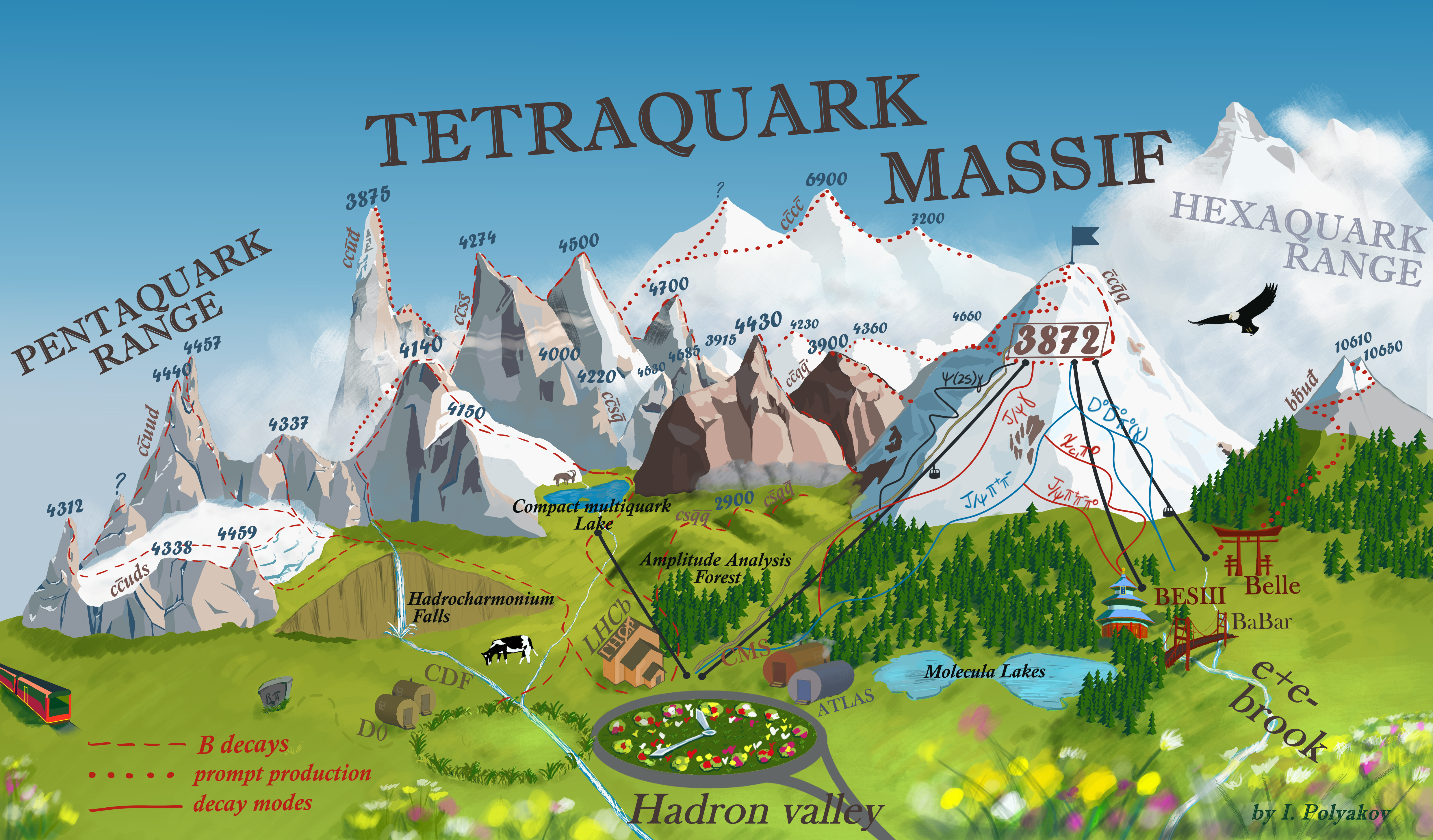
The exotic-hadron landscape

Exotic hadron experimental studies, illustration by I. Polyakov

Backup

Tcc⁺ structure

Backup: Tcc⁺, two extreme spatial configurations
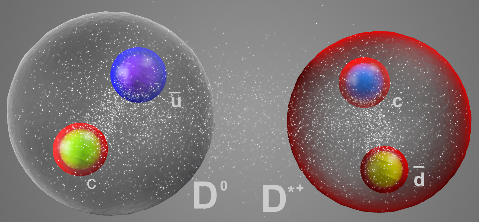
Molecular picture: D⁰ and D*⁺ mesons well separated, exchanging light mesons
Molecule: D⁰ and D*⁺ held by π, ρ, … exchange
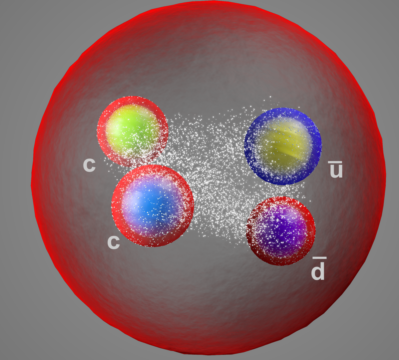
Compact picture: cc diquark with ūd̄ in one hadron
Compact: a (cc) core with ū d̄

Molecular configuration

Two mesons, well separated, bound like van der Waals forces. Entirely coupled to D*⁺D⁰; the lifetime is limited by the D*⁺. Spatially extended.

Compact configuration

A genuine QCD state with a compact (cc) core, about 1 fm. The lifetime depends on how strongly it couples to the continuum.