Getting started

This page takes one calculation through every step: load the model, pick a meson, compute its spectrum, read one state, and look at its wavefunction. Later pages explain each step in more depth.

Installation

GIModel needs Julia 1.11 or later. It is not yet registered, so add it from GitHub:

using Pkg
Pkg.add(url = "https://github.com/mmikhasenko/GIModel.jl")

For a local checkout, use Pkg.develop(path = "/path/to/GIModel.jl"). The package has four external dependencies (KrylovKit, PartialWaveFunctions, QuadGK and SpecialFunctions) and no plotting or file-format dependencies.

Step 1: load the model

The model is a set of numbers taken from the paper: quark masses, the confinement slope and offset, smearing widths, and relativistic factors. They ship with the package as a TOML file.

using GIModel
params, mq = load_parameters_and_quark_masses(default_parameters_path())
mq

Dict{String, Float64} with 6 entries:
  "c" => 1.628
  "b" => 4.977
  "u" => 0.22
  "q" => 0.22
  "s" => 0.419
  "d" => 0.22

params is a GIParameters object holding the interaction. mq is a QuarkMassTable with constituent masses in GeV. They are kept separate on purpose: the interaction is flavor-blind, and quark masses enter only through the meson you build.

Step 2: choose a meson

A Meson is a quark–antiquark pair. The first flavor is the quark, the second is the antiquark:

charmonium = Meson(mq, :c, :c)

Meson: c cbar   (m1 = 1.628, m2 = 1.628 GeV, reduced = 0.814 GeV)
  self-conjugate: same-J antisymmetric spin-orbit mixing vanishes

Meson(mq, :c, :s) would be the system (the family), and Meson(mq, :q, :q) uses the averaged light mass for and .

Step 3: choose which levels to compute

States are labeled  : radial quantum number , total quark spin , orbital angular momentum , and total angular momentum . spectrum_levels lists all of them up to a radial number:

levels = spectrum_levels(1; L_labels = ("S", "P"))
[level.label for level in levels]

6-element Vector{String}:
 "1^1S_0"
 "1^3S_1"
 "1^1P_1"
 "1^3P_0"
 "1^3P_1"
 "1^3P_2"

Step 4: compute the spectrum

spectrum = compute_spectrum(params, charmonium; levels = spectrum_levels(2))

MixedSpectrum: cc, 20 levels — all values in GeV
  level     central    contact   fine str     mixing       mass
  1^1S_0     3.0784    -0.1117     0.0000     0.0000     2.9667
  1^3S_1     3.0656     0.0256     0.0000    -0.0002     3.0910
  2^1S_0     3.6665    -0.0411     0.0000     0.0000     3.6254
  2^3S_1     3.6661     0.0127     0.0000    -0.0000     3.6788
  1^1P_1     3.5232    -0.0082     0.0000     0.0000     3.5151
  1^3P_0     3.5348     0.0037    -0.0957     0.0000     3.4428
  1^3P_1     3.5238     0.0028    -0.0185     0.0000     3.5082
  1^3P_2     3.5248     0.0022     0.0211     0.0000     3.5481
  2^1P_1     3.9625    -0.0064     0.0000     0.0000     3.9561
  2^3P_0     3.9641     0.0025    -0.0503     0.0000     3.9163
  2^3P_1     3.9625     0.0022    -0.0116     0.0000     3.9531
  2^3P_2     3.9631     0.0018     0.0145     0.0000     3.9794
  1^1D_2     3.8384    -0.0019     0.0000     0.0000     3.8366
  1^3D_1     3.8405     0.0007    -0.0231     0.0001     3.8182
  1^3D_2     3.8385     0.0006    -0.0018     0.0000     3.8373
  1^3D_3     3.8391     0.0006     0.0081     0.0000     3.8477
  2^1D_2     4.2091    -0.0016     0.0000     0.0000     4.2075
  2^3D_1     4.2101     0.0006    -0.0168     0.0001     4.1941
  2^3D_2     4.2091     0.0005    -0.0015     0.0000     4.2081
  2^3D_3     4.2095     0.0005     0.0065     0.0000     4.2165
  (4 levels carry mixing; see `spec.states[i].mixings`)

Each row is a level. The columns are in GeV and add up to the mass:

column	meaning
central	the spin-independent energy: kinetic term, confinement and Coulomb, plus the quark masses
contact	the spin–spin contact (hyperfine) interaction
fine str	spin–orbit plus tensor, diagonal in the level
mixing	the shift from mixing with other levels of the same
mass	the physical meson mass

All contributions are evaluated in the same eigenstate, which is why they sum exactly to the mass. The last line says that some levels carry mixing: here the tensor force mixes with .

Step 5: look at one state

spectrum_state picks a level by its label:

chi_c1 = spectrum_state(spectrum, "1^3P_1")
chi_c1.mass_GeV

3.5081502109538754

The state also carries its quantum numbers and every contribution:

(chi_c1.n, chi_c1.L, chi_c1.multiplicity, chi_c1.J)

(1, "P", 3, 1)

(central = chi_c1.central_GeV,
 spin_orbit = chi_c1.spin_orbit_shift_GeV,
 tensor = chi_c1.tensor_shift_GeV,
 contact = chi_c1.contact_shift_GeV)

(central = 3.5238043169507294, spin_orbit = -0.028732806502261746, tensor = 0.010230059107934618, contact = 0.002848641397473027)

Step 6: get its wavefunction

For a level that does not mix, radial_wave returns the radial wavefunction:

eta_c = radial_wave(spectrum, "1^1S_0")
wave_norm(eta_c)

0.9999999999999999

The is slightly mixed with the states, so it has more than one component. physical_components returns all of them, each with a signed coefficient and its own radial wave:

[(c.basis.label, round(c.coefficient; digits = 4))
 for c in physical_components(spectrum, "1^3S_1")]

4-element Vector{Tuple{String, Float64}}:
 ("1^3S_1", 0.9999)
 ("2^3S_1", -0.0)
 ("1^3D_1", -0.0133)
 ("2^3D_1", 0.0086)

Asking radial_wave for a mixed state throws an error. That is deliberate: a mixed state has no single radial wave, so the package does not return one.

The mean-square radius and momentum come from wave_mean_squares, in and :

wave_mean_squares(eta_c, 0)

(r2 = 2.1229942234941013, p2 = 1.2899911969232778)

To plot the wave, sample it on a grid of radii in :

using CairoMakie
r = range(0, 12; length = 241)
fig = Figure(size = (600, 320))
ax = Axis(fig[1, 1]; xlabel = "r  [GeV⁻¹]", ylabel = "u(r)")
for label in ("1^1S_0", "2^1S_0", "1^1P_1")
    wave = sample_wave(radial_wave(spectrum, label), r)
    lines!(ax, wave.r, wave.u; label)
end
axislegend(ax)
fig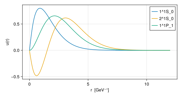

Here u(r) is the reduced radial wavefunction, normalized as   .

Step 7: use the paper’s numerical method

compute_spectrum uses a fast finite-difference solver by default. Godfrey and Isgur expanded the wavefunctions in harmonic-oscillator functions instead. Pass an OscillatorSolver to use that method:

ho = compute_spectrum(params, charmonium;
    levels = spectrum_levels(1; L_labels = ("S",)), solver = OscillatorSolver())

MixedSpectrum: cc, 2 levels — all values in GeV
  level     central    contact   fine str     mixing       mass
  1^1S_0     3.0785    -0.1114     0.0000     0.0000     2.9671
  1^3S_1     3.0658     0.0256     0.0000     0.0000     3.0914

The two methods agree to a fraction of an MeV. The oscillator solver also checks its own convergence; Solvers and convergence explains both solvers.

Where to go next

• The model writes out the Hamiltonian behind these numbers.

• Computing a spectrum covers level selection, the stages of the calculation, and switching spin terms on and off.

• Wavefunctions covers wave representations, momentum space and mixed states.

• Charmonium, start to finish continues this example with radiative and leptonic decays.