Wavefunctions

Every state in a spectrum carries its wavefunction. Decays, radii and annihilation widths are all computed from it, so this page explains how wavefunctions are represented and how to work with them.

using GIModel
params, mq = load_parameters_and_quark_masses(default_parameters_path())
spec = compute_spectrum(params, Meson(mq, :c, :c);
    levels = spectrum_levels(2), solver = OscillatorSolver())

The radial wavefunction

For a state with orbital angular momentum , the position-space wavefunction factorizes as

where is the quark–antiquark separation in and is the reduced radial wavefunction. GIModel always works with .

Two representations

The abstract type RadialWave has two concrete forms, one per solver:

• OscillatorWave: coefficients of an expansion in harmonic-oscillator functions with scale , plus .

• MeshWave: samples on a uniform mesh.

eta_c = radial_wave(spec, "1^1S_0")
(typeof(eta_c), eta_c.L, eta_c.beta, length(eta_c.coefficients))

(OscillatorWave, 0, 1.126393202250021, 40)

Code that uses a wave should not depend on which form it has. The operations below work for both, so the same analysis runs with either solver.

Operations

operation	computes
wave_norm(w)	(1 for solver output)
radial_expect(w, f)
radial_overlap(w1, w2, f)
wave_mean_squares(w, L)	and
momentum_wave(w, L)	the momentum-space wave
momentum_expect(Φ, g)
momentum_overlap(Φ1, Φ2, g)
sample_wave(w, r)	samples on a grid, for plotting or export

radial_expect(eta_c, r -> r^2)          # ⟨r²⟩ in GeV⁻²

2.1260095433986588

psi2S = radial_wave(spec, "2^1S_0")
radial_overlap(eta_c, psi2S, r -> 1.0)  # orthogonal radial states

-4.878912886550984e-16

wave_mean_squares(eta_c)                # (r2 in GeV⁻², p2 in GeV²)

(r2 = 2.1260095433986588, p2 = 1.2869039978250068)

Convert with   GeV fm: the root-mean-square separation of the is    fm.

Smooth functions integrate best. For oscillator waves, radial_expect evaluates \int u^2 f\,dr by Gauss–Laguerre quadrature in x = (\beta r)^2. Even powers of r are exact. Functions like r or 1/r are not polynomials in x; they converge more slowly and may emit a quadrature warning. The warning reports what was reached rather than hiding it.

Plotting wavefunctions

sample_wave evaluates any radial wave on a grid of radii and returns a MeshWave with fields r and u:

using CairoMakie
r = range(0, 10; length = 301)
fig = Figure(size = (700, 300))
ax1 = Axis(fig[1, 1]; xlabel = "r  [GeV⁻¹]", ylabel = "u(r)", title = "reduced radial wave")
ax2 = Axis(fig[1, 2]; xlabel = "r  [GeV⁻¹]", ylabel = "u(r)²", title = "radial probability")
for label in ("1^1S_0", "2^1S_0", "1^1P_1", "2^1P_1")
    w = sample_wave(radial_wave(spec, label), r)
    lines!(ax1, w.r, w.u; label)
    lines!(ax2, w.r, w.u .^ 2)
end
axislegend(ax1; position = :rt)
fig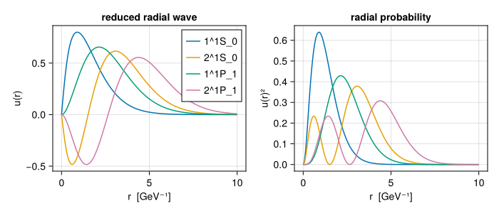

Each radial excitation adds a node. All waves use the same sign convention: the outermost lobe is positive (see Conventions and units).

Momentum space

The momentum-space radial wave is the spherical Bessel transform

For an oscillator wave the transform is exact; for a mesh wave it is computed numerically on a momentum grid (pmax, npoints). A mesh wave does not store , so pass it explicitly:

Φ = momentum_wave(eta_c)
momentum_expect(Φ, p -> p^2)             # ⟨p²⟩ in GeV²

1.2869039978250068

For an oscillator wave, evaluate the analytic momentum wave directly to plot it:

fig = Figure(size = (450, 300))
ax = Axis(fig[1, 1]; xlabel = "p  [GeV]", ylabel = "p Φ(p)")
for label in ("1^1S_0", "2^1S_0", "1^1P_1")
    w = radial_wave(spec, label)
    Φs = momentum_wave(w)
    p = range(0, 4; length = 400)
    lines!(ax, p, p .* Φs.(p); label)
end
axislegend(ax)
fig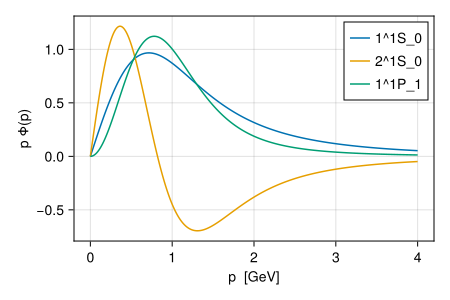

The relativistic kinetic energy matters because these distributions reach  .

Mixed states

A mixed state is a superposition of basis states, each with its own radial wave, so it has no single u(r). radial_wave refuses it:

try
    radial_wave(spec, "1^3S_1")
catch err
    println(sprint(showerror, err))
end

ArgumentError: 1^3S_1 is a mixed physical state; use physical_components instead of selecting one precursor radial wave

physical_components returns the full decomposition. Each component is a named tuple with the pure basis state, its signed coefficient, and its native wave:

components = physical_components(spec, "1^3S_1")
[(c.basis.label, round(c.coefficient; digits = 4), typeof(c.wave)) for c in components]

4-element Vector{Tuple{String, Float64, DataType}}:
 ("1^3S_1", 0.9999, OscillatorWave)
 ("2^3S_1", -0.0, OscillatorWave)
 ("1^3D_1", -0.0133, OscillatorWave)
 ("2^3D_1", 0.0086, OscillatorWave)

The squared coefficients sum to one:

sum(abs2(c.coefficient) for c in components)

1.0

The decomposition is recursive. For an isoscalar that has gone through spectroscopic mixing and then annihilation mixing, physical_components multiplies through both steps and returns flavor-tagged components; see Isoscalar flavor mixing.

For an unmixed state, physical_components returns one component with coefficient 1, so code written with it works for every state.

Coherent amplitudes

Physical amplitudes are linear in the state: an amplitude for a mixed state is the coefficient-weighted sum of the amplitudes of its components, with signs. physical_state_amplitude performs this sum. You write a kernel for one pure component, without its coefficient:

# An illustrative linear amplitude: overlap of each S-wave component with η_c through r².
kernel(c) = c.basis.L_label == "S" ? radial_overlap(eta_c, c.wave, r -> r^2) : 0.0
physical_state_amplitude(kernel, spec, "1^3S_1")

2.426785248375888

Transition matrix elements in Transitions and decays are built this way, so interference between components is always kept.

Before mixing

radial_wave(spec, state.corrected) returns the wave of the assigned basis state before mixing. This is useful for diagnostics, but it is not the physical state.