Strong decays beyond the paper

Godfrey and Isgur computed strong decays    with the elementary-emission operator of Eq. (19). For their Table V they used one simplification: every meson got the same Gaussian wavefunction, with   GeV. GIModel can instead evaluate the same operator between the solved wavefunctions, each with its own size, radial nodes and mixing. This tutorial builds the states, fixes the two couplings, and predicts decays that were not used in the fit.

using GIModel
using GIModel.QuarkModelTransitions
params, mq = load_parameters_and_quark_masses(default_parameters_path())
solver = OscillatorSolver()

The operator

A quark or antiquark in the parent emits a pseudoscalar with momentum ; is the momentum of the emitting quark. The direct coupling and the recoil coupling (both in ) are phenomenological. The amplitude is linear in them, so two numbers fitted to data fix every decay.

Building the states

Solve the flavor channels we need. Each BasisState is a level to keep:

S1, S0 = BasisState(1, "S", 3, 1), BasisState(1, "S", 1, 0)
P1_triplet, P1_singlet = BasisState(1, "P", 3, 1), BasisState(1, "P", 1, 1)
solve(f1, f2, levels) = compute_spectrum(params, Meson(mq, f1, f2); levels, solver)
ud = solve(:u, :d, [S1, S0, P1_triplet, P1_singlet])
uu, dd = solve(:u, :u, [S1, S0]), solve(:d, :d, [S1, S0])
us, ds = solve(:u, :s, [S1, S0]), solve(:d, :s, [S0])

Charged states come straight from their spectra:

rho, pi_plus, a1, b1 = (physical_state(ud, b) for b in (S1, S0, P1_triplet, P1_singlet))
K_star, K_plus, K_zero = physical_state(us, S1), physical_state(us, S0), physical_state(ds, S0)
(ρ = rho.mass_GeV, a₁ = a1.mass_GeV, b₁ = b1.mass_GeV, K⁺ = K_plus.mass_GeV)

(ρ = 0.7712488094493981, a₁ = 1.2375460303738788, b₁ = 1.2184697225583834, K⁺ = 0.4612729692037647)

Neutral isospin states are superpositions of and . superpose combines the solved states and normalizes their coherent wavefunction. The model has degenerate u and d masses, so the component masses are equal here; the resulting mass is supplied explicitly:

up0, down0 = physical_state(uu, S0), physical_state(dd, S0)
up1, down1 = physical_state(uu, S1), physical_state(dd, S1)
pi_zero = superpose([up0, down0], [1, -1]; label="π⁰", mass_GeV=up0.mass_GeV)
omega = superpose([up1, down1], [1, 1]; label="ω", mass_GeV=up1.mass_GeV)
pi_zero

PhysicalState("π⁰", 0.14906372897241119 GeV, 2 components)

The flavor components must be explicit (:u, :d): the averaged :q cannot say whether a state is   or  , so the operator rejects it.

Channels

A TwoMesonChannel is ordered as (surviving, emitted), and the emitted meson must be a pseudoscalar:

channels = [
    "ρ⁺ → π⁺ π⁰" => (TwoMesonChannel(pi_plus, pi_zero), rho),
    "K*⁺ → K⁰ π⁺" => (TwoMesonChannel(K_zero, pi_plus), K_star),
    "K*⁺ → K⁺ π⁰" => (TwoMesonChannel(K_plus, pi_zero), K_star),
    "a₁⁺ → ρ⁺ π⁰" => (TwoMesonChannel(rho, pi_zero), a1),
    "b₁⁺ → ω π⁺" => (TwoMesonChannel(omega, pi_plus), b1),
]
amplitude(name, g, h) = matrix_element(first(Dict(channels)[name]),
    PseudoscalarEmission(g, h, mq), last(Dict(channels)[name]))

For two pseudoscalars in the final state, as in  , either one could be called the emitted meson. The operator evaluates the assignment you give and never adds the other one silently.

Fixing the couplings

The ratio . In the paper’s single-Gaussian limit the Table IV amplitudes reduce to two combinations,    and  . The paper’s fit gives  , which fixes the ratio:

r = 3.291 / 1.644
h_over_g = r / (3 - r / 4)

0.8008760722759628

The scale. Fix so that    MeV. Since the width is quadratic in the couplings, one evaluation at   is enough:

unit_width = decay_width(amplitude("ρ⁺ → π⁺ π⁰", 1.0, h_over_g))
g = sqrt(149.1 / unit_width)
h = h_over_g * g
(g = g, h = h)

(g = 3.555583210811114, h = 2.8475815165247615)

Predictions

for (name, _) in channels
    a = amplitude(name, g, h)
    waves = partial_waves(a)
    line = rpad(name, 14) * "q = $(round(Int, 1000a.momentum_GeV)) MeV   Γ = $(round(decay_width(a); digits = 1)) MeV"
    if length(waves) == 2
        line *= "   D/S = $(round(real(a[waves[2]] / a[waves[1]]); digits = 3))"
    end
    println(line)
end

ρ⁺ → π⁺ π⁰    q = 356 MeV   Γ = 149.1 MeV
K*⁺ → K⁰ π⁺   q = 312 MeV   Γ = 58.7 MeV
K*⁺ → K⁺ π⁰   q = 312 MeV   Γ = 29.3 MeV
a₁⁺ → ρ⁺ π⁰   q = 358 MeV   Γ = 234.3 MeV   D/S = -0.14
b₁⁺ → ω π⁺    q = 343 MeV   Γ = 120.9 MeV   D/S = 0.256

Compare with measured values:

decay	model	measured
	sum of the two lines above	MeV
		(isospin)
, D/S	see above
, D/S	see above
	see above	MeV ( dominant)

The D/S ratios test the internal structure of the P-wave mesons and do not depend on the overall scale . The ratio is reproduced well, and the ratio has the measured sign. The width is overestimated: the ratio came from the paper’s Gaussian-wavefunction fit, and the decay momentum uses the model masses, which are a few MeV off.

Kinematics use model masses

Momenta and widths above use the masses of the solved states: the model pion is 149 MeV rather than 138 MeV, and the model is 902 MeV rather than 892 MeV. mass_correction_factor shows how an amplitude would change at the measured momentum, keeping the wavefunctions fixed:

a = amplitude("K*⁺ → K⁰ π⁺", g, h)
wave = only(partial_waves(a))
factor = mass_correction_factor(first(Dict(channels)["K*⁺ → K⁰ π⁺"]),
    PseudoscalarEmission(g, h, mq), K_star; target_momentum = 0.291, partial_wave = wave)

0.9370022218084451 - 0.0im

The factor multiplies that partial-wave amplitude; the phase-space factor in the width changes separately.

How the couplings enter

Because the amplitude is linear in and , the D/S ratio of an axial meson depends only on . Scanning it shows how sensitive each ratio is:

using CairoMakie
ratios = range(0.0, 1.6; length = 41)
d_over_s(name, x) = (a = amplitude(name, 1.0, x); w = partial_waves(a); real(a[w[2]] / a[w[1]]))
fig = Figure(size = (500, 320))
ax = Axis(fig[1, 1]; xlabel = "h / g", ylabel = "D / S")
lines!(ax, ratios, [d_over_s("b₁⁺ → ω π⁺", x) for x in ratios]; label = "b₁ → ωπ")
lines!(ax, ratios, [d_over_s("a₁⁺ → ρ⁺ π⁰", x) for x in ratios]; label = "a₁ → ρπ")
vlines!(ax, [h_over_g]; color = :gray, linestyle = :dash)
axislegend(ax; position = :lt)
fig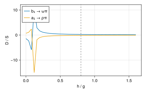

The dashed line is the ratio from the paper’s fit. A global fit of and to several widths and ratios would be the next step for a quantitative study.

What this operator is, and is not

The emitted pion is treated as an elementary field: its mass and flavor enter, but its wavefunction is not integrated. This is the Godfrey–Isgur emission model, not a quark-pair-creation () model. It cannot describe decays that need a new quark pair, such as   through creation, or decays into two non-pseudoscalar mesons. See Scope and limitations.