Charmonium, start to finish
This tutorial carries out a complete study of one system: the charmonium spectrum, where each mass comes from, what the states look like, and their radiative, leptonic and annihilation widths. It uses the pieces introduced in the Manual; each step links back to the relevant page.
using GIModel
using GIModel.QuarkModelTransitions
using CairoMakie
params, mq = load_parameters_and_quark_masses(default_parameters_path())
charmonium = Meson(mq, :c, :c)
1. The spectrum
We use the paper’s oscillator method and compute S, P and D waves up to the second radial excitation:
spec = compute_spectrum(params, charmonium;
    levels = spectrum_levels(2), solver = OscillatorSolver())
MixedSpectrum: cc, 20 levels — all values in GeV
level central contact fine str mixing mass
1^1S_0 3.0785 -0.1114 0.0000 0.0000 2.9671
1^3S_1 3.0658 0.0256 0.0000 -0.0002 3.0912
2^1S_0 3.6668 -0.0410 0.0000 0.0000 3.6258
2^3S_1 3.6664 0.0127 0.0000 -0.0000 3.6791
1^1P_1 3.5233 -0.0082 0.0000 0.0000 3.5151
1^3P_0 3.5348 0.0037 -0.0956 0.0000 3.4429
1^3P_1 3.5239 0.0028 -0.0185 0.0000 3.5082
1^3P_2 3.5248 0.0022 0.0211 0.0000 3.5482
2^1P_1 3.9626 -0.0064 0.0000 0.0000 3.9562
2^3P_0 3.9643 0.0025 -0.0502 0.0000 3.9165
2^3P_1 3.9627 0.0022 -0.0116 0.0000 3.9532
2^3P_2 3.9632 0.0018 0.0145 0.0000 3.9795
1^1D_2 3.8385 -0.0019 0.0000 0.0000 3.8366
1^3D_1 3.8405 0.0007 -0.0231 0.0001 3.8183
1^3D_2 3.8385 0.0006 -0.0018 0.0000 3.8374
1^3D_3 3.8391 0.0006 0.0081 0.0000 3.8477
2^1D_2 4.2092 -0.0016 0.0000 0.0000 4.2075
2^3D_1 4.2102 0.0006 -0.0168 0.0001 4.1941
2^3D_2 4.2092 0.0005 -0.0015 0.0000 4.2082
2^3D_3 4.2095 0.0005 0.0065 0.0000 4.2166
(4 levels carry mixing; see `spec.states[i].mixings`)Compare the states below the open-charm threshold with their measured masses (PDG averages, rounded to 1 MeV):
measured = [
    "1^1S_0" => ("η_c(1S)", 2.984), "1^3S_1" => ("J/ψ", 3.097),
    "1^3P_0" => ("χ_c0", 3.415), "1^3P_1" => ("χ_c1", 3.511),
    "1^1P_1" => ("h_c", 3.525), "1^3P_2" => ("χ_c2", 3.556),
    "2^1S_0" => ("η_c(2S)", 3.638), "2^3S_1" => ("ψ(2S)", 3.686),
    "1^3D_1" => ("ψ(3770)", 3.774),
]
for (label, (name, m_exp)) in measured
    m = spectrum_state(spec, label).mass_GeV
    println(rpad(name, 9), rpad(label, 8), "model ", round(m; digits = 3),
        "  measured ", m_exp, "  Δ = ", round(Int, 1000 * (m - m_exp)), " MeV")
end
η_c(1S) 1^1S_0 model 2.967 measured 2.984 Δ = -17 MeV
J/ψ 1^3S_1 model 3.091 measured 3.097 Δ = -6 MeV
χ_c0 1^3P_0 model 3.443 measured 3.415 Δ = 28 MeV
χ_c1 1^3P_1 model 3.508 measured 3.511 Δ = -3 MeV
h_c 1^1P_1 model 3.515 measured 3.525 Δ = -10 MeV
χ_c2 1^3P_2 model 3.548 measured 3.556 Δ = -8 MeV
η_c(2S) 2^1S_0 model 3.626 measured 3.638 Δ = -12 MeV
ψ(2S) 2^3S_1 model 3.679 measured 3.686 Δ = -7 MeV
ψ(3770) 1^3D_1 model 3.818 measured 3.774 Δ = 44 MeVA level diagram shows the pattern at a glance. Each column is one
columns = [
    ("0⁻⁺", "1^1S_0", [2.984, 3.638]), ("1⁻⁻", "1^3S_1", [3.097, 3.686]),
    ("0⁺⁺", "1^3P_0", [3.415]), ("1⁺⁺", "1^3P_1", [3.511]),
    ("1⁺⁻", "1^1P_1", [3.525]), ("2⁺⁺", "1^3P_2", [3.556]),
]
fig = Figure(size = (650, 380))
ax = Axis(fig[1, 1]; ylabel = "mass  [GeV]",
    xticks = (1:length(columns), [c[1] for c in columns]))
for (x, (_, label, masses)) in enumerate(columns)
    ground = spectrum_state(spec, label)
    for n in 1:2
        m = spectrum_state(spec, n, ground.L, ground.multiplicity, ground.J).mass_GeV
        lines!(ax, [x - 0.3, x + 0.3], [m, m]; color = :black)
    end
    scatter!(ax, fill(x, length(masses)), masses; color = :tomato, markersize = 10)
end
hlines!(ax, [3.730]; linestyle = :dash, color = :gray)
text!(ax, 0.6, 3.74; text = "D D̄ threshold", fontsize = 11, color = :gray)
fig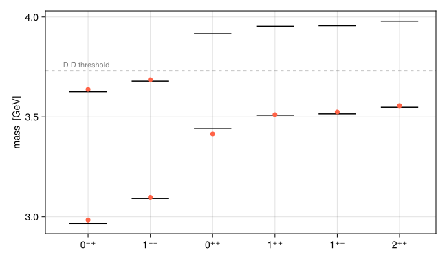
2. Where the masses come from
The spectrum table already splits each mass. The pattern is worth reading closely:
The contact term pushes
down by about 110 MeV and up by about 25 MeV. With identical wavefunctions the ratio would be the In P waves, the contact term is small but nonzero: smearing gives the contact interaction a finite range.
The fine structure orders the
as
Split the
for J in 0:2
    s = spectrum_state(spec, "1^3P_$J")
    println("χ_c$J   vector SO ", round(1000s.spin_orbit_vector_shift_GeV; digits = 1),
        "   Thomas ", round(1000s.spin_orbit_thomas_shift_GeV; digits = 1),
        "   tensor ", round(1000s.tensor_shift_GeV; digits = 1), "  (MeV)")
end
χ_c0 vector SO -94.6 Thomas 22.8 tensor -23.8 (MeV)
χ_c1 vector SO -39.8 Thomas 11.1 tensor 10.2 (MeV)
χ_c2 vector SO 33.6 Thomas -10.7 tensor -1.8 (MeV)The one-gluon (vector) spin-orbit term and the Thomas precession from confinement have opposite signs. The tensor shifts roughly follow the ratio
To see a term’s total effect, switch it off and recompute (Computing a spectrum). Without the spin-orbit and tensor terms, the three
no_fine = compute_spectrum(params, charmonium;
    levels = spectrum_levels(1; L_labels = ("P",)), solver = OscillatorSolver(),
    terms = SpinTerms(fine_structure = false))
[s.label => round(s.mass_GeV; digits = 4) for s in no_fine.states]
4-element Vector{Pair{String, Float64}}:
"1^1P_1" => 3.5151
"1^3P_0" => 3.5256
"1^3P_1" => 3.5256
"1^3P_2" => 3.52563. What the states look like
r = range(0, 10; length = 301)
fig = Figure(size = (700, 300))
ax = Axis(fig[1, 1]; xlabel = "r  [fm]", ylabel = "u(r)²  [GeV]")
for label in ("1^1S_0", "2^1S_0", "1^1P_1", "1^1D_2")
    w = sample_wave(radial_wave(spec, label), r)
    lines!(ax, w.r .* 0.1973, w.u .^ 2; label)
end
axislegend(ax)
fig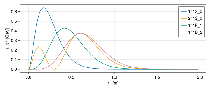
for label in ("1^1S_0", "2^1S_0", "1^1P_1", "1^1D_2")
    w = radial_wave(spec, label)
    m = wave_mean_squares(w)
    println(rpad(label, 8), "√⟨r²⟩ = ", round(sqrt(m.r2) * 0.1973; digits = 3), " fm   ",
        "√⟨p²⟩ = ", round(sqrt(m.p2); digits = 3), " GeV   ",
        "v²/c² ≈ ", round(m.p2 / (m.p2 + mq["c"]^2); digits = 2))
end
1^1S_0 √⟨r²⟩ = 0.288 fm √⟨p²⟩ = 1.134 GeV v²/c² ≈ 0.33
2^1S_0 √⟨r²⟩ = 0.639 fm √⟨p²⟩ = 1.118 GeV v²/c² ≈ 0.32
1^1P_1 √⟨r²⟩ = 0.52 fm √⟨p²⟩ = 0.98 GeV v²/c² ≈ 0.27
1^1D_2 √⟨r²⟩ = 0.702 fm √⟨p²⟩ = 1.0 GeV v²/c² ≈ 0.27The
The
[(c.basis.label, round(c.coefficient; digits = 4)) for c in physical_components(spec, "1^3S_1")]4-element Vector{Tuple{String, Float64}}:
("1^3S_1", 0.9999)
("2^3S_1", -0.0)
("1^3D_1", -0.0133)
("2^3D_1", 0.0086)The tensor force admixes
4. Radiative transitions
The photon operators of the paper connect S waves with S waves (M1) and with P waves (E1, M2). In the spectrum above, the PhotonEmission would refuse them. For radiative transitions we therefore solve the S and P waves only, as the paper does for its Table VI. Here we use a separate S/P spectrum:
radiative = compute_spectrum(params, charmonium;
    levels = spectrum_levels(2; L_labels = ("S", "P")), solver = OscillatorSolver())
Resolve the states once as PhysicalStates:
state(label) = physical_state(radiative, label)
psi, psi2S, eta_c = state("1^3S_1"), state("2^3S_1"), state("1^1S_0")
photon = PhotonEmission(mq)
The E1 transitions between S and P waves are the strongest radiative decays of charmonium:
for J in 0:2
    chi = state("1^3P_$J")
    down = decay_width(matrix_element(psi, photon, chi))
    up = decay_width(matrix_element(chi, photon, psi2S))
    println("χ_c$J → J/ψ γ: ", round(1000down; digits = 1), " keV     ",
        "ψ(2S) → χ_c$J γ: ", round(1000up; digits = 1), " keV")
end
χ_c0 → J/ψ γ: 128.9 keV ψ(2S) → χ_c0 γ: 14.6 keV
χ_c1 → J/ψ γ: 210.4 keV ψ(2S) → χ_c1 γ: 22.7 keV
χ_c2 → J/ψ γ: 268.4 keV ψ(2S) → χ_c2 γ: 21.5 keVThe E1 width scales as
Magnetic dipole transitions flip the quark spin. Between states of the same radial level (DirectM1) they are small; between different levels (HinderedM1) they would vanish without relativistic corrections and wavefunction differences:
direct = matrix_element(eta_c, photon, psi)
hindered = matrix_element(eta_c, photon, psi2S)
(direct = (direct.transition_class, round(1000decay_width(direct); digits = 2)),
 hindered = (hindered.transition_class, round(1000decay_width(hindered); digits = 2)))
(direct = (GIModel.QuarkModelTransitions.DirectM1(), 2.36), hindered = (GIModel.QuarkModelTransitions.HinderedM1(), 0.78))Widths are in keV. The hindered transition is weaker even though its photon momentum is five times larger, because its overlap nearly cancels.
5. Leptonic and annihilation widths
These widths depend on the wavefunction near the origin:
current = LeptonicCurrent(:electromagnetic, mq)
two_photon = TwoPhotonAnnihilation(mq, AnnihilationTerm((:c, :c), 4 / 9))
gluons = GluonicAnnihilation(mq, M -> alpha_s_q(M))
(ψ_ee = 1000decay_width(MasslessLeptonPair(), current, psi),
 ψ2S_ee = 1000decay_width(MasslessLeptonPair(), current, psi2S),
 ηc_γγ = 1000decay_width(TwoPhotonChannel(), two_photon, eta_c),
 ηc_gg = decay_width(TwoGluonChannel(), gluons, eta_c))
(ψ_ee = 10.511053477744904, ψ2S_ee = 3.5329994712630834, ηc_γγ = 7.525020971568651, ηc_gg = 24.583472509534875)The first three are in keV, the last in MeV. The ratio
6. Is it converged?
The oscillator solver certifies the energies (see Solvers and convergence). A width is a different quantity, so check it directly with the independent finite-difference solver:
fd = compute_spectrum(params, charmonium; levels = spectrum_levels(2; L_labels = ("S", "P")),
    solver = FiniteDifferenceSolver(ngrid = 1200))
compare(label_i, label_f) = (
    decay_width(matrix_element(physical_state(radiative, label_f), photon, physical_state(radiative, label_i))),
    decay_width(matrix_element(physical_state(fd, label_f), photon, physical_state(fd, label_i))))
for (i, f) in (("1^3P_1", "1^3S_1"), ("2^3S_1", "1^3P_2"), ("1^3S_1", "1^1S_0"))
    ho_w, fd_w = compare(i, f)
    println(rpad("$i → $f", 20), "HO ", round(1000ho_w; digits = 3), " keV   FD ",
        round(1000fd_w; digits = 3), " keV")
end
1^3P_1 → 1^3S_1 HO 210.421 keV FD 210.412 keV
2^3S_1 → 1^3P_2 HO 21.521 keV FD 21.507 keV
1^3S_1 → 1^1S_0 HO 2.364 keV FD 2.365 keVThe two methods agree, so the widths are properly converged.
Summary
In a few calls we obtained the charmonium spectrum with its decomposition, the wavefunctions, and a set of decay widths, and checked convergence with a second method. The same steps work for any flavor combination: Heavy-light mesons and mixing repeats them for a system where singlet–triplet mixing matters.